Decision Trees

Can be seen multipe ways:

As a function
Both input and output can be discrete or continuous.
$f:$ vector $\vec x$ of attribute values $\mapsto$ a single output value called decision
Can be any function of the input attributes.

As a binary tree
decision is reached by performing a sequence of tests (from root to leaf).
Edges: possible value $v_{i,k}$ of the input attributes $A_i$
Leafs: possible decisions

Goal: Finding a tree that is consistent with the examples and as small as possible.

Each training set has a consistent decision tree: one path to leaf for each example but it won’t generalize to new examples.

We want to learn the most compact tree.

We can not efficiently search through $2^{2^n}$ trees.

But there are simple heuristics to find a good approximate solution.

A more expressive hypothesis space $\mathcal H$ :

$+$ increases the chance that target function can be expressed

$-$ but the hypotheses consistent with the training set may get worse predictions.

Learning a good hypothesis

We want a small, flat decision tree with subsets that are all positive or negative.

Examples (Training Set)

Set of $(\vec x, y)$ pairs where $\vec x$ are the input attributes and $y$ are the decisions (boolean output).

Decision-Tree-Learning DTL

Greedy divide-and-conquer algorithm: queue sorted by the "most important attribute".

/*
- examples: (x, y) pairs
- attributes: attributes of values x_1, x_2, ... x_n in x in example
- classification: y_j = true / false
*/function DTL(examples, attributes, parent_examples) returns a decision tree
if examples is empty then return MAJORITY(parent_examples.classifications)
else if all examples have the same classification then return the classification
else if attributes is empty then return MAJORITY(examples.classification)
else
A = empty
for each Attribute A' do
A ← maxImportance(A, A', examples)tree ← a new decision tree with root test Afor each (value v of A) do //all possible values from domain of A
exs ← {e : e ∈ examples | e.A = v} //all examples where this value occured
subtree ← DTL(exs, attributes\{A}, examples) //recursive call
add a new branch to tree with label "A = v" and subtree subtreereturn tree

The algorithm is recursive, every sub tree is an independent problem with fewer examples and one less attribute.

The returned tree is not identical to the correct function / tree $f$ . It is a hypothesis $h$ based on examples.

no examples left
then it means that there is no example with this combination of values → We return a default value: the majority function on examples in the parents.

Remaining examples are all positive or negative
we are done

no attributes left but both positive and negative examples
These examples have the same description but different classifications, we return the plurality-classification (Reasons: noise in data, non determinism)

some positive or negative examples
choose the most important attribute to split and repeat this process for subtree

Defining importance

We choose the attribute with most importance - Which attribute is the best predictor for the classification?

The one with the highest information gain.

Entropy

Information gain measured with entropy

Entropy measures uncertainty of the occurence of a random variable in [shannon] or [bit].

Entropy of a random variable $A$ with values $v_k$ each with probability $P(v_k)$ is defined as:

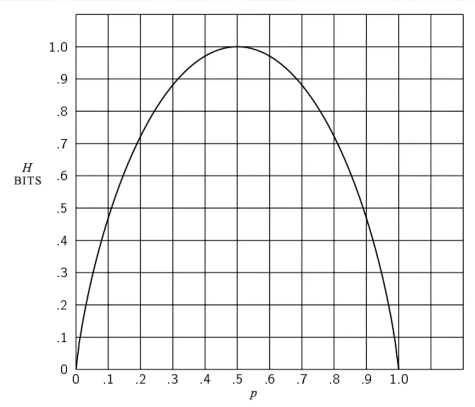
H(A)=∑kP(vk)log⁡2(1P(vk))=−∑kP(vk)log⁡2(P(vk))H(A) = \sum_k P(v_k)\log_2 \biggl( \frac{1}{P(v_k)} \biggl)= - \sum_k P(v_k)\log_2(P(v_k))H(A)=k∑P(vk)log2(P(vk)1)=−k∑P(vk)log2(P(vk))

Entropy is at its maximum when all outcomes are equally likely.

💡

With lower entropy, we can ask fewer questions to get to a decision.

Entropy of a boolean random variable

Boolean random variable $V$ : Variable is true with probability $q$ and false with $(1-q)$ .

Same formula as above.

B(q)=−(q⋅log⁡2(q)+(1−q)⋅log⁡2(1−q))B(q)=-(q\cdot \log_2(q)+(1-q)\cdot \log_2(1-q))B(q)=−(q⋅log2(q)+(1−q)⋅log2(1−q))

Entropy of the goal attribute

If a training set contains $p$ positive and $n$ negative examples then the entropy of the goal attribute on the whole set is

B(P(reachinggoal))=B(pp+n)B(~P(reaching \space goal)~) = B \biggl(\frac{p}{p+n} \biggl)B(P(reachinggoal))=B(p+np)

Remainder

Entropy remaining after testing a single attribute.

We treat each attribute $A$ like a random variable with $d$ possible subsets for each value.

Each value occurs in $p_k$ positive and $n_k$ negative training set examples. (index $k$ stands for the subset we are currently in).

The probability that specific value occuring (based on our the training set):

P(randomly chosen example containsvk)=pk+nkp+nP(\text{randomly chosen example contains} ~v_k)= \frac{p_k+n_k}{p+n}P(randomly chosen example containsvk)=p+npk+nk

Therefore the expected entropy remaining after testing the attribute $A$ is:

Remainder(A)=∑k=1dpk+nkp+n⋅B(pkpk+nk)Remainder(A) = \sum^d_{k=1} \frac{p_k + n_k}{p+n} \cdot B \biggl(\frac{p_k}{p_k + n_k} \biggl)Remainder(A)=k=1∑dp+npk+nk⋅B(pk+nkpk)

Gain

Information gain from an attribute → defines importance.

The information gain from an attribute is the reduction of its entropy after testing.

Gain(A)=B(pp+n)−Remainder(A)Gain(A)=B \biggl( \frac{p}{p+n} \biggl) -Remainder(A)Gain(A)=B(p+np)−Remainder(A)

Where $Gain(A)$ defines how many questions we need to ask on average until we reach a decision.

Rem vs. Gain

💡

We either choose the lowest entropy / remainder value for an attribute, or the highest gain.

Rem and gain contradict eachother

Rem tells us the randomness / distribution of data

Gain tells us the usefulness of data

Our goal is to reach a decision with the fewest number of required tests.

Broadening the applicability of decision trees

While extending the applicability of decision trees a number of issues arise.

Missing data

Often not all the attributes are known in every example. → consider all possible values, weighted with frequency to reach the test node (by the examples)

Multivalued attributes

When an attribute has many possible values, then the information gain measure gives an inappropriate indication of the usefulness. → use gain ratio, test different values at different tree heights, normalize the gain with the entropy of $A$

Continuous and integer-valued input attributes

Instead of branching infinitely use split points (Age > 35) with the highest information gain.

(Splitting is the most expensive part of real-world decision tree learning applications)

Continuous-valued output attributes

For numerical predictions like prices: regression trees whose leaves are functions of a subset of the attributes.