Informed Search
Algorithms
Heuristic / Best First Search BFS algorighms use problem/domain-specific knowledge during search.
(unknown) true total cost from to goal
Evaluation function - estimation for , used for node expansion
Path cost from start to .
Heuristic function - estimated cost of the cheapest path from .
Function can not be computed from the problem itself.
Computing it must have a low cost.
Output must be at the goal node.
Greedy BFS
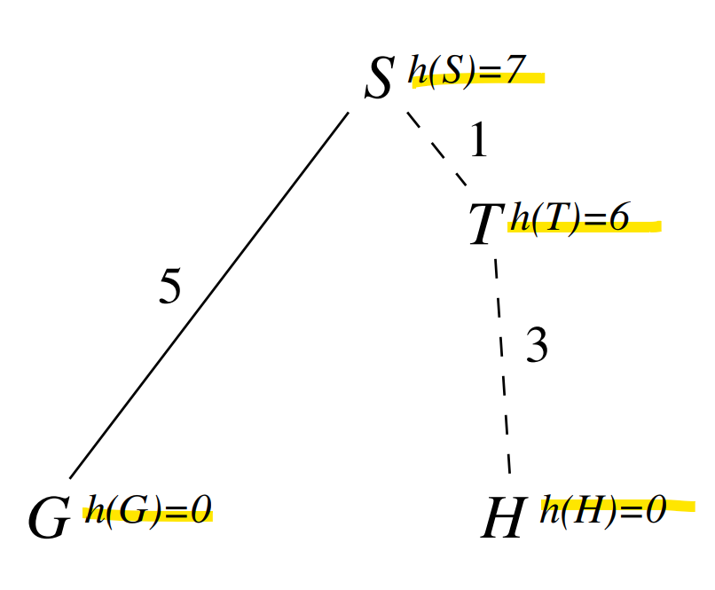
Just like UCS but instead of for the priority queue ordering - does not take already spent costs into account.
completeness No - only in finite state spaces with explored set
time complexity
space complexity
optimality of solution No
A* Search
Solves non-optimality and possibility of non-termination of greedy search.
Just like UCS - but for the priority queue.
where heuristic must be admissible.
completeness Yes - with finite nodes and , costs , step-costs
time complexity where is the effective branching factor with rel. error .
space complexity Exponential, keeps all nodes in memory
optimality of solution Yes
admissible for tree-search is optimal (proof)
start node
optimal goal node
non goal node
unexpanded node on optimal path to
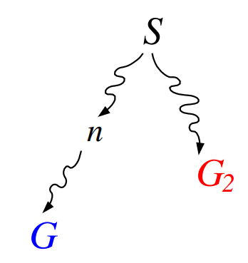
Since there are no unexpanded nodes to
Because is suboptimal
(cost to , and to goal)
Because the heuristic is admissible
Therefore A* will never select
consistent for graph search is optimal
If decreases during optimal path to goal it is discarded by graph-search.
(But in tree search it is not a problem since there is only a single path to the optimal goal).
Solutions to problem:
- consistency of (non decreasing on every path)
- additional book-keeping
optimal efficiency Yes
A* expands the fewest nodes possible - no other optimal algorithm can expand fewer nodes than A* because not expanding nodes with runs the risk of missing the optimal solution.
Relationship to Dijkstras Algorithm
Shortest path from one node to all nodes in a graph. (There are 2 variants: shortest path from one node to all nodes - or - all nodes to all nodes)
Uses no heuristics, made for a finite and explicit graph.
Uses - can be seen as a UCS algorithm or as a special case of A* where .
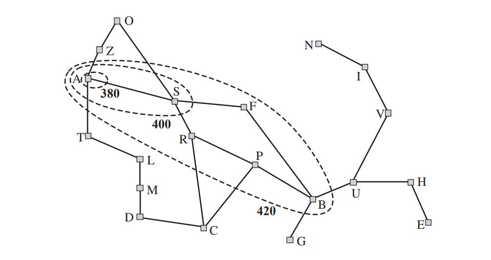
Contours in the state space
Because -costs are nondecreasing along any path we can draw contours in the state space, just like the contours in a topographic map.
With uniform-cost search, the bands will be "circular" around the start state.
With more accurate heuristics, the bands will stretch toward the goal state and become more narrowly focused around the optimal path.
Heuristics
Admissibility
Optimistic, never overestimating, never negative.
goals: (follows from the above)
Deriving admissible heuristics
from exact solution cost of a relaxed version of the problem.
Because the optimal solution cost of a relaxed problem is than the optimal solution cost of the real problem. The relaxation should be polynomially computable.
Examples
Examples: 8-puzzle
- Rules are relaxed so that a tile can move anywhere: gives the shortest solution
- Rules are relaxed so that a tile can move to any adjacent square: gives the shortest solution
Example: Traveling salesman problem TSP
"Find the shortest tour visiting all cities exactly once."
View all cities as a Graph where each Vertice must be connected .
The Minimum spanning tree MST is a lower bound for this problem that can be calculated with Kruskal and Prim
Example: shortest path
straight airline-distance between two destinations
Consistency / Monotonicity
Every consistent heuristic is also admissible. Consistency is stricter than admissibility.
Implies that -value is non-decreasing on every path .
For every node and its successor :
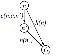
This is a form of the general triangle inequality.
is then non-decreasing along every path:
(because of consistency)
Dominance
For two admissible heuristics, we say dominates , if:
Then is better for search.
Local Search
For many (also optimization) problems, paths are irrelevant, only the solution matters.
The aim is an iterative improvement .
We define our state space: set of "complete" but not optimal configurations:
- keep a single "current" state - (constant space usage)
- try to improve it until goal state is reached - (optimal configuration)
Examples
Examples: unknown environments (online search), TSP, constraint satisfaction problems,
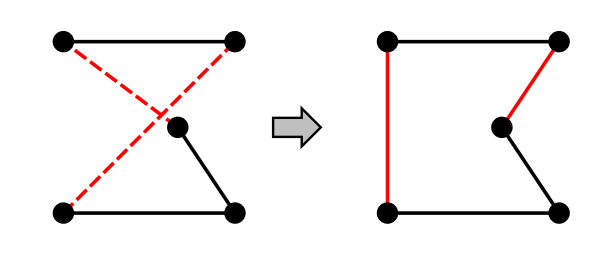
Traveling Salesman Problem TSP
Variants of this approach get within 1% of optimal very quickly with thousands of cities
Pairwise exchange of crossing paths:
- start with any complete tour
- perform pairwise exchanges
n-queens
Move a queen to reduce number of conflicts (attacks), e.g., in column
Terminates in few steps (at most quadratic, but much fewer in reality)

Greedy local search
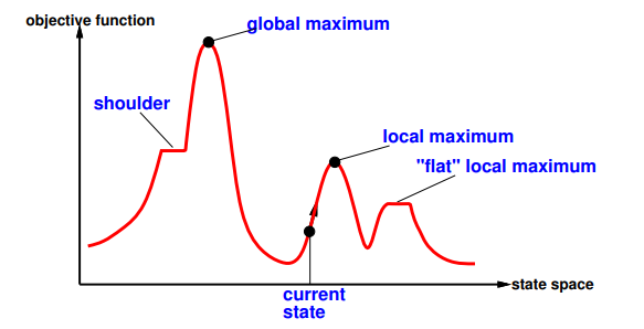
Also called "hill-climbing":
escaping shoulders
getting stuck in loop at local maximum
Solution: Random-restart hill climbing: restart after step limit overcomes local maxima
Pseudocode
function HILL-CLIMBING(problem) returns a state that is a local maximum
inputs: problem // a problem
local variables:
current, // a node
neighbor // a node
current ← MAKE-NODE(INITIAL-STATE[problem])
loop do
neighbor ← a highest-valued successor of current
if VALUE[neighbor] ≤ VALUE[current] then return STATE[current]
current ← neighbor
Simulated annelaing
Devised in the 1950s for physical process modeling.
Corresponds to "cooling off" process of materials
In depth
- value = energy
- Based on Boltzmann distribution: If is decreased slowly enough: reach best (lowest energy) state with probability approaching , for small
- The slower this process is, the better the results
Idea: Escaping local maxima by gradually allowing less "bad" moves in size and frequency.
Problem: "Slowly enough" can be worse than exhaustive search.
Pseudocode
function SIMULATED-ANNEALING(problem, schedule) returns a solution state
inputs:
problem, //a problem
schedule, //a mapping from time to “temperature”
local variables: current, //a node
next, //a node
T, //a “temperature” controlling prob. of downward steps
current ← MAKE-NODE(INITIAL-STATE[problem])
for t ← 1 to ∞ do
T ← schedule[t]
if T = 0 then return current
next ← a randomly selected successor of current
∆E ← VALUE[next] – VALUE[current]
if ∆E > 0 then current ← next
else current ← next only with probability e∆E/T
Local beam search
Idea
- keep states instead of just to start searching from
- Not running searches in parallel: Searches that find good states recruit other searches to join them
- choose top of all their successors
Problem
often, all states end up on same local hill
Solution
choose successors randomly, biased towards good ones
Genetic algorithms GA
Stochastic local beam search + successors from pairs of states
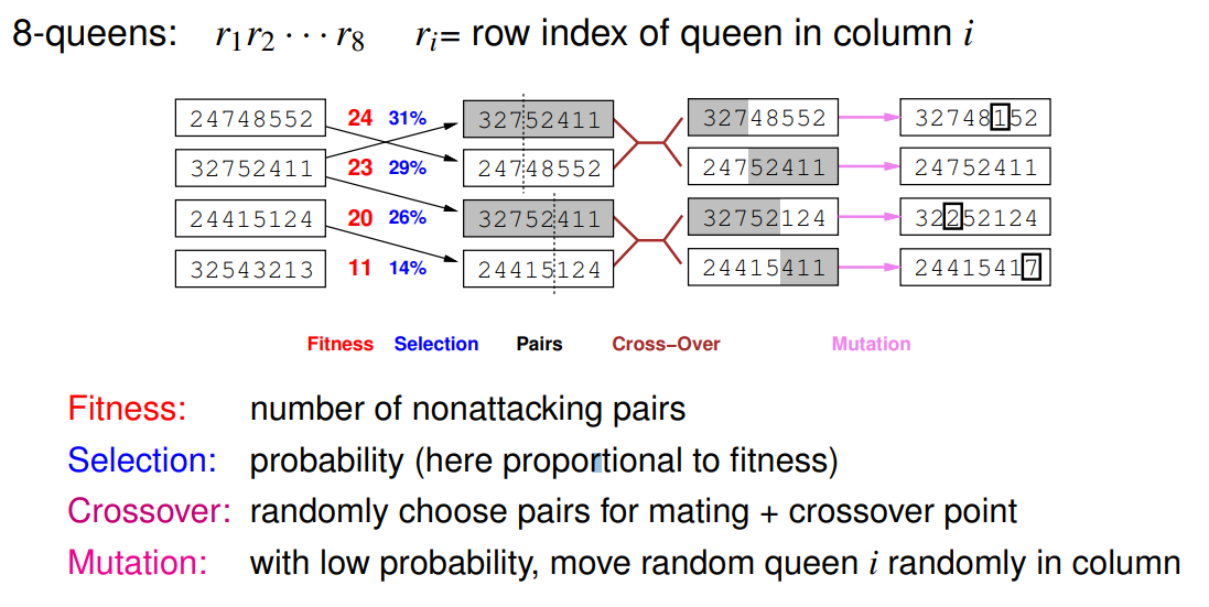
- GAs require states encoded as strings (lists of instructions as individuals)
- Crossover can produce solutions quite distant from their parents → Crossover helps if and only if substrings are meaningful components (blocks) (not random shuffling)

