Linear Classification

💡

This is not part of the curriculum - just here to show that perceptrons are actually linear classifiers.

Hard threshold

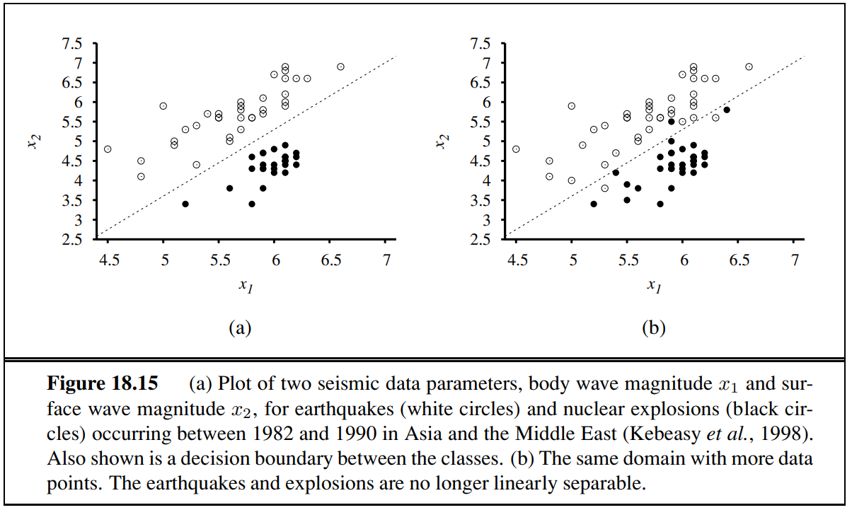
A decision boundary is a line (or a surface, in higher dimensions) that separates two classes. Then line then is called a linear separator.

Example
Given these training data, the task of classification is to learn a hypothesis $h$ that will take new $(x_1, x_2)$ points and return either $0$ for earthquakes or $1$ for explosions.

Using the convention of a dummy input $x_0 = 1$ we can write the classification hypothesis as:

g(x)=hw(x)={1,ifw⋅x≥00,otherwiseg(\mathbf{x}) = h_{\mathbf{w}}(\mathbf{x}) = \begin{cases} 1,& \text{if } \mathbf{w} \cdot \mathbf{x}\geq 0\\ 0, & \text{otherwise} \end{cases}g(x)=hw(x)={1,0,ifw⋅x≥0otherwise

Alternatively one could see it as a threshold function where $\vec w \cdot \vec x$ is the threshold $t$ .

We want to choose the weights to minimize the loss.

Previously in linear regression we did this both in closed form (by setting the gradient to zero and solving for the weights) and by gradient descent in weight space (hill climb algorithm).

Now we cannot do either of those things because the gradient is zero almost everywhere in weight space except at those points where $\vec w \cdot \vec x = 0$ , and at those points the gradient is undefined.

Perceptron learning rule

Weight update rule that converges to the optimal solution most of the time (a linear separator that classifies the data perfectly if data is linearly seperable) - but very slowly.

wi←wi+α(y−hw⃗(x⃗))⋅xiw_i \larr w_i + \alpha(y-h_{\vec w}(\vec x)) \cdot x_iwi←wi+α(y−hw(x))⋅xi

For multiple examples: Applied like in stochastic gradient decent for each individual weight:

We only consider a single randomly chosen example at a time with the equation for single training examples.

More efficient, can be done online with data constantly coming in - however, it does not guarantee convergence. It can oscillate around the minimum without settling down.

How does exactly it work?

We have our currect output $h_{\vec w}$ and the output of the examples $y \in \{0,1\}$ with a given $\vec x$ .

$y = h_{\vec w}(\vec x)$
Our weights are correct. $w_i$ stays unchanged.

$y=1$ and $h_{\vec w}(\vec x) = 0$
Our weights are incorrect. We want to make $h_{\vec w}(\vec x) = 1$
If $x_i$ is positive $\rarr w_i$ gets increased
If $x_i$ is negative $\rarr w_i$ gets decreased

$y=0$ and $h_{\vec w}(\vec x) = 1$
Our weights are incorrect. We want to make $h_{\vec w}(\vec x) = 0$
If $x_i$ is positive $\rarr w_i$ gets decreased
If $x_i$ is negative $\rarr w_i$ gets increased

Soft threshhold

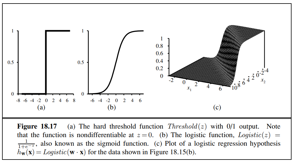
The previous hypothesis $h_{\vec w}(\vec x)$ is not differentiable, discontinuous, very unpredictable.

It also always announces a completely confident prediction of 1 or 0, even for examples that are very close to the boundary - we often want more granularity in predictions.

We therefore now want to use the sigmoid funcion $g$ . It converges slower than the hard threshold but behaves a lot more predictable.

g(x)=hw(x)=Logistic⁡(w⋅x)=11+e−w⋅xg(\mathbf{x}) = h_{\mathbf{w}}(\mathbf{x})=\operatorname{Logistic}(\mathbf{w} \cdot \mathbf{x})=\frac{1}{1+e^{-\mathbf{w} \cdot \mathbf{x}}}g(x)=hw(x)=Logistic(w⋅x)=1+e−w⋅x1

Notice that the output, being a number between 0 and 1, can be interpreted as a probability of belonging to the class labeled 1.

Logistic Regression

The process of fitting the weights of this model to minimize loss on a data set is called logistic regression.

There is no easy closed-form solution to find the optimal value of $\vec w$ → Search for minimal loss by gradient descent:

We can use the $\text{Loss}$ function again because our hypotheses $\not\in \{0,1\}$ .

Loss⁡(w)=(y−hw(x))2\operatorname{Loss}(\mathbf{w}) =\left(y-h_{\mathbf{w}}(\mathbf{x})\right)^{2}Loss(w)=(y−hw(x))2

One training example

Because of the chain rule for $g(f(x))$ :

$\partial g(f(x)) / \partial x=g^{\prime}(f(x)) \cdot \partial f(x) / \partial x$

∂∂wiLoss⁡(w)=∂∂wi(y−hw(x))2=2(y−hw(x))⋅∂∂wi(y−hw(x))=−2(y−hw(x))⋅g′(w⋅x)⋅∂∂wiw⋅x=−2(y−hw(x))⋅g′(w⋅x)⋅xi\begin{aligned}\frac{\partial}{\partial w_{i}} \operatorname{Loss}(\mathbf{w}) &=\frac{\partial}{\partial w_{i}}\left(y-h_{\mathbf{w}}(\mathbf{x})\right)^{2} \\&=2\left(y-h_{\mathbf{w}}(\mathbf{x})\right) \cdot \frac{\partial}{\partial w_{i}}\left(y-h_{\mathbf{w}}(\mathbf{x})\right) \\&=-2\left(y-h_{\mathbf{w}}(\mathbf{x})\right) \cdot g^{\prime}(\mathbf{w} \cdot \mathbf{x}) \cdot \frac{\partial}{\partial w_{i}} \mathbf{w} \cdot \mathbf{x} \\&=-2\left(y-h_{\mathbf{w}}(\mathbf{x})\right) \cdot g^{\prime}(\mathbf{w} \cdot \mathbf{x}) \cdot x_{i}\end{aligned}∂wi∂Loss(w)=∂wi∂(y−hw(x))2=2(y−hw(x))⋅∂wi∂(y−hw(x))=−2(y−hw(x))⋅g′(w⋅x)⋅∂wi∂w⋅x=−2(y−hw(x))⋅g′(w⋅x)⋅xi

The derivative $g'$ of the logistic function satisfies

g(z)=g(z)(1−g(z))g(z) = g(z)(1 − g(z))g(z)=g(z)(1−g(z))

so we have

g′(w⋅x)=g(w⋅x)(1−g(w⋅x))=hw(x)(1−hw(x))g^{\prime}(\mathbf{w} \cdot \mathbf{x})=g(\mathbf{w} \cdot \mathbf{x})(1-g(\mathbf{w} \cdot \mathbf{x}))=h_{\mathbf{w}}(\mathbf{x})\left(1-h_{\mathbf{w}}(\mathbf{x})\right)g′(w⋅x)=g(w⋅x)(1−g(w⋅x))=hw(x)(1−hw(x))

g′(w⋅x)=hw(x)(1−hw(x))g^{\prime}(\mathbf{w} \cdot \mathbf{x})= h_{\mathbf{w}}(\mathbf{x})\left(1-h_{\mathbf{w}}(\mathbf{x})\right)g′(w⋅x)=hw(x)(1−hw(x))

so the weight update for minimizing the loss is

wi←wi+α(y−hw(x))⋅hw(x)(1−hw(x))⋅xiw_{i} \leftarrow w_{i}+\alpha\left(y-h_{\mathbf{w}}(\mathbf{x})\right) \cdot h_{\mathbf{w}}(\mathbf{x})\left(1-h_{\mathbf{w}}(\mathbf{x})\right) \cdot x_{i}wi←wi+α(y−hw(x))⋅hw(x)(1−hw(x))⋅xi