Exam on 2016-06-28

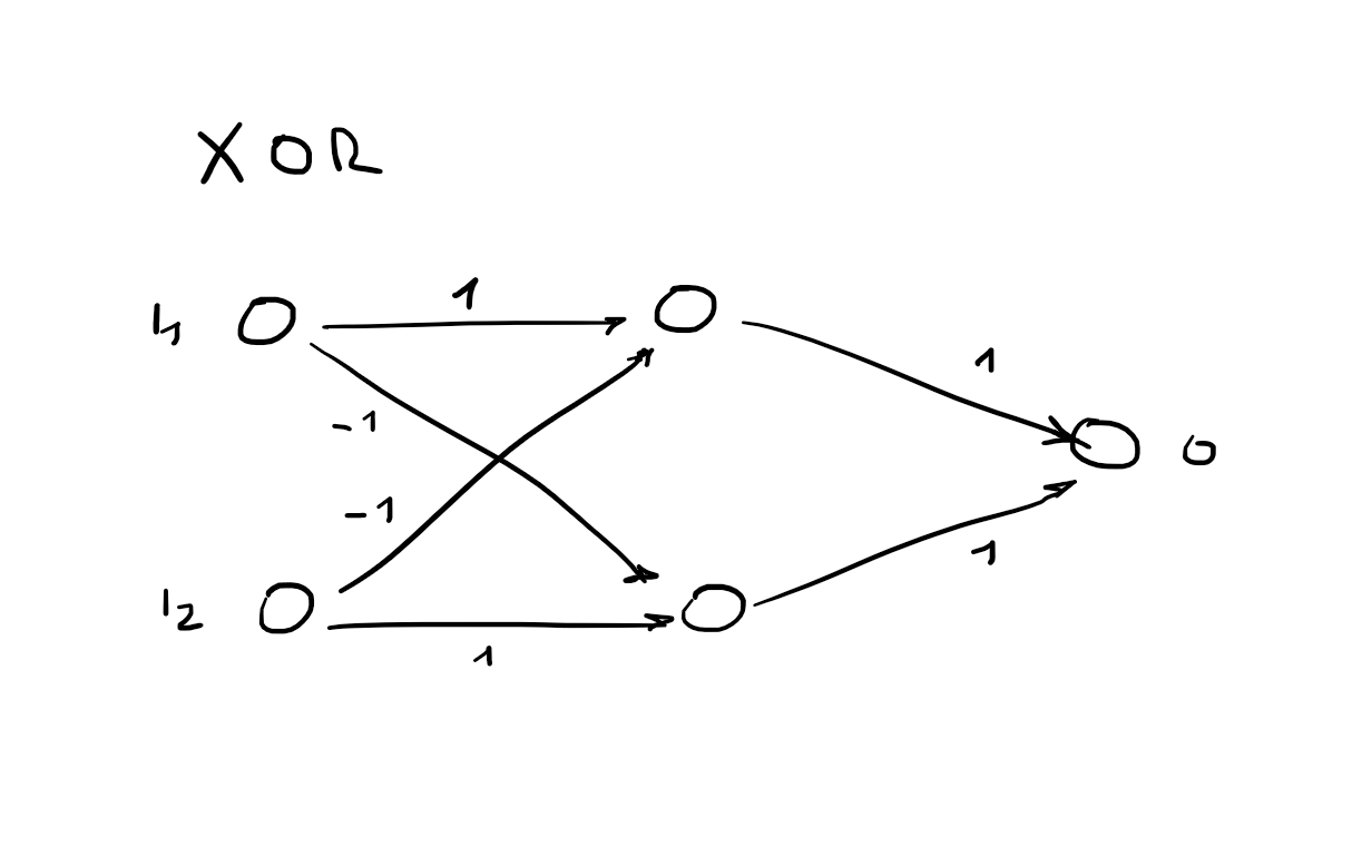
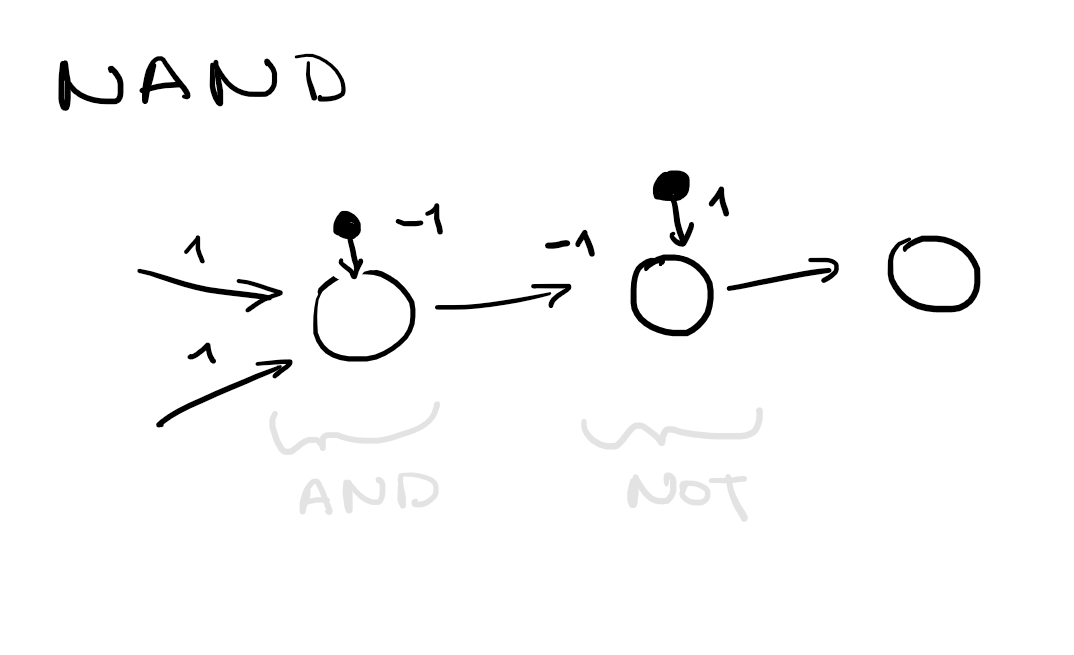
After_Test_-_28.06.2016_-_Einfhrung_in_die_Knstliche_Intelligenz_VU_-_Informatik-Forum_der_TU_Wien.pdf

1. Construct a neural network

2 inputs

2 outputs: nand, xor

Activation function:

$g(x)=\left\{\begin{array}{ll}1 & \text { if } x \geq 1, \\0 & \text { otherwise }\end{array}\right.$

2. Explain the local beam search and mention its advantages / disadvantages

Idea keep $k$ states instead of just $1$

Not the same as running $k$ searches in parallel: Searches that find good states recruit other searches to join them - choose top $k$ of all their successors

Problem often, all $k$ states end up on same local hill

Solution choose $k$ successors randomly, biased towards good ones

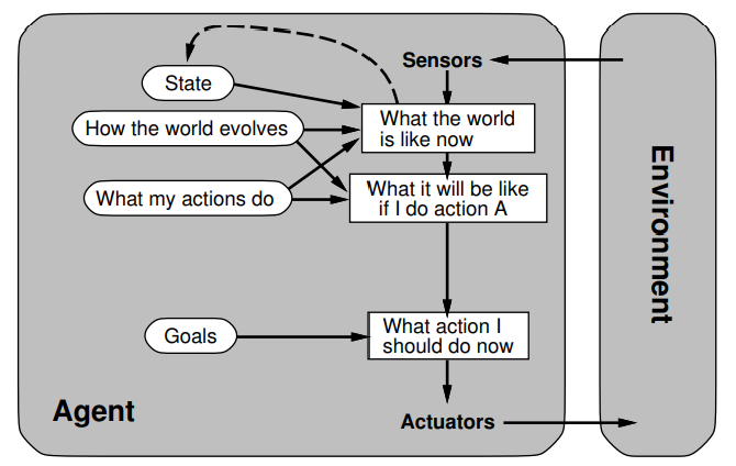
3. Describe the components of the goal-based agent

Add on: explicit goals , ability to plan into the future, model outcomes for predictions

model the world , goals, actions and their effects explicitly

more flexible, better maintainability

Search and planning of actions to achieve a goal

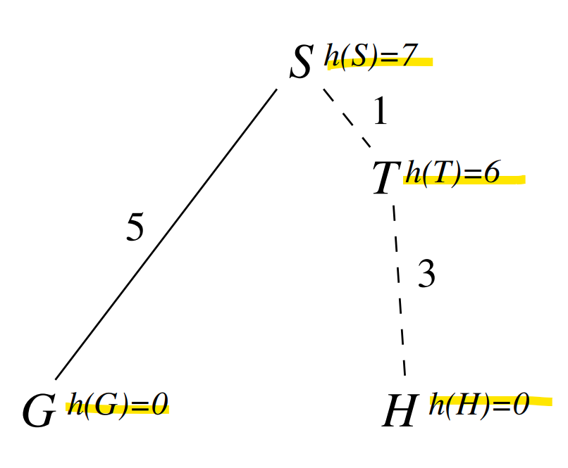
4. Use the A* search

on a small graph

which nodes get expanded?
nodes where $f(n) \leq C^*$

what do the costs look like?
$f(n) = g(n) + h(n)$ where heuristic must be admissible.

Is BFS a special case of A*?
No it isnt, BFS uses a queue but A* search uses a priority queue.

A* Search

Solves non-optimality and possibility of non-termination of greedy search.

Just like UCS - but $g+h$  for the priority queue.

$f(n) = g(n) + h(n)$ where heuristic must be admissible.

completeness Yes - with finite nodes and $b$ , costs $\leq C^*$ , step-costs $\geq \varepsilon$

time complexity $O(b^{\varepsilon d})$ where $b^\varepsilon$ is the effective branching factor with rel. error $\varepsilon = \frac{h - f^*}{f^*}$ .

space complexity Exponential, keeps all nodes in memory

optimality of solution Yes

non admissible $h(n)$ for tree-search is not optimal (proof)
$S \dots$ start node
$G,H\dots$ goal nodes
We immedeately expand non-optimal goal $G$ because $h(G) = 0$ although $f(G) = 5+0$ .
Then we check $f(T) = 6+1$ and terminate search.

admissible $h(n)$ for tree-search is optimal (proof)
$S\dots$ start node
$G\dots$ optimal goal node
$G_2\dots$ non goal node
$n\dots$ unexpanded node on optimal path to $G$
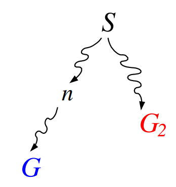
Since there are no unexpanded nodes to $G_2$
$f(G_2) = g(G_2) + h(G_2)$
$f(G_2) = g(G_2) + 0$
Because $G_2$ is suboptimal
$\textcolor{grey}{f(G_2) =} g(G_2) > g(G) \textcolor{grey}{= g(n)+ f^*(n)}$ (cost to $n$ , and $n$ to goal)
$f(G_2) > g(n)+ f^*(n)$
Because the heuristic is admissible
$f(G_2) > g(n)+ f^*(n) \geq g(n)+ h(n)\textcolor{grey}{= f(n)}$
$f(G_2) > f(n)$
Therefore A* will never select $G_2$

consistent $h(n)$ for graph search is optimal
If $h(n)$ decreases during optimal path to goal it is discarded by graph-search.
(But in tree search it is not a problem since there is only a single path to the optimal goal).
Solutions to problem:
- consistency of $h$ (non decreasing $f$ on every path)
- additional book-keeping

optimal efficiency Yes

A* expands the fewest nodes possible - no other optimal algorithm can expand fewer nodes than A* because not expanding nodes with $f(n) < C^*$ runs the risk of missing the optimal solution.

5. Multiple choice

What are the decisions of an rational agent based on?

Decisions based on evidence:

percept history

built-in knowledge of the environment - ie. fundamental knowledge laws like physics

BFS expands as many nodes as DFS

No - BFS uses a queue and DFS uses a stack.

BFS time complexity $O(b^d)$

Goal test at generation time: $1 + b + b^2 + b^3 + ... + b^d = O(b^d)$

Goal test at expansion time: $1 + b + b^2 + b^3 + ... + b^d + \textcolor{pink}{b^{d+1}}= O(b^{d+1})$

DFS time complexity $O(b^m)$ - where maximum depth $m$ may be $\infin$

IDS is optimal for limited tree depth

Yes- but also for unknown tree depths

it has solution optimality if step cost ≥ 1

In general IDS is very attractive and prefered when the search space is large and the depth of the solution is unknown.

It is usually only a little more expensive than BFS.

STRIPS only allows disjunctions in goals

No it doesnt - only conjunctions

ADL supports the notation for equaliy / inequality

Yes

6. Constraint graphs

3 coloring problem - geographical map - draw a constraint graph

7. Heuristics for backtracking search

Variable ordering: fail first

Minimum remaining (legal) values MRV

degree heuristic - (used as a tie breaker), variable that occurs the most often in constraints

Value ordering: fail last

least-constraining-value - a value that rules out the fewest choices for the neighbouring variables in the constraint graph.

8. Explain the value of information - Can it be calculated without additional information?

Value of Information

$\text{value = }(\text{ avg. best action before obtaining}) - (\text{avg. best action after obtaining})$

Value of perfect information VPI(= expected value of information)

Can be used if we do not have additional information - we then just use averages

Lets say the exact evidence $e_j$ (= perfect information) of the random variable $E_j$ is currently unknown.

We define:

Best action $\alpha$ before learning $e_j = E_j$ under all actions $\textcolor{pink}a$

$E U(\alpha \mid \mathbf{e})=\max _{\textcolor{pink}a} \sum_{s^{\prime}} P(\operatorname{RESULT}(\textcolor{pink}a)=s^{\prime} \mid \textcolor{pink}a, \mathbf{e}) \cdot U(s^{\prime})$

Best action $\alpha_{e_j}$ after learning $e_j = E_j$ under all actions $\textcolor{pink}a$

$E U(\alpha_{e_{j}} \mid \mathbf{e}, e_{j})=\max _{\textcolor{pink}a} \sum_{s^{\prime}} P(\operatorname{RESULT}(\textcolor{pink}a)=s^{\prime} \mid \textcolor{pink}a, \mathbf{e}, e_{j}) \cdot U(s^{\prime})$

Value of learning the exact evidence is the cost of discovering it for ourselves under $\mathbf{e}$ by averaging over all possible values $e_{jk}$ of $E_j$ .

VPIe(Ej)=(∑kP(Ej=ejk∣e)⋅EU(αejk∣e,Ej=ejk))−EU(α∣e)V P I_{\mathbf{e}}(E_{j})=\left(\sum_{k} P(E_{j}=e_{j k} \mid \mathbf{e}) \cdot EU(\alpha_{e_{j k}} \mid \mathbf{e}, E_{j}=e_{j k})\right)-E U(\alpha \mid \mathbf{e})VPIe(Ej)=(k∑P(Ej=ejk∣e)⋅EU(αejk∣e,Ej=ejk))−EU(α∣e)

9. Explain the estimated utility, maximum estimated utility

Utility function

$U(s)$ desireability of state

Expected Utility (average utility value)

Its impicit that $s'$ can follow from the current state $s$ .

$E U(a \mid \mathbf{e})=\sum_{s^{\prime}} P(\operatorname{RESULT}(a)=s^{\prime} \mid a, \mathbf{e}) \cdot U(s^{\prime})$

Sum of: Probability of state occuring after action times its utility

Principle of maximum expected utility MEU

rational agent should choose the action that maximizes the agents expected utility

$\text { action }=\underset{a}{\operatorname{argmax}} \space E U(a \mid \mathbf{e})$

10. Construct a STRIPS action

Install a software

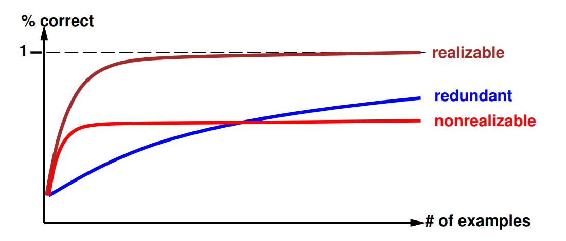
11. Explain the learning curve and mention reasons for its non-optimality

How do we know that $h ≈ f$ ? (Hume’s Problem of Induction)

Learning curve = % correct on test set when using $h$

Learning curve depends on realizability of the target function.

Non-realizability can be due to

missing attributes

too restrictive hypothesis space (e.g.,linear function)

redundant expressiveness (e.g., loads of irrelevant attributes)