Exam on 2018-06-26

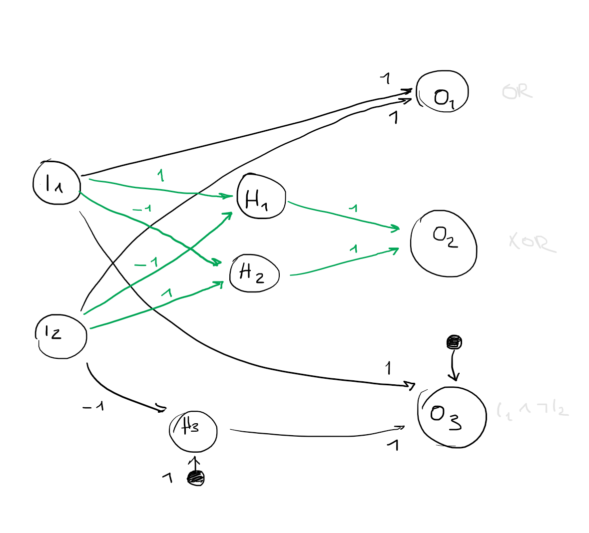
TU_Wien-Einfhrung_in_die_Knstliche_Intelligenz_VU_(Eiter_Tompits)_-_Prfung_2018-06-26.pdf

Part 1)

a) Construct a neural network

Properties:

max 1 inner layer

2 binary inputs $I_1, I_2$

3 outputs $O_1, O_2, O_3$

$\begin{array}{c|c||c|c|c}I_{1} & I_{2} & O_{1} & O_{2} & O_{3} \\\hline 0 & 0 & 0 & 0 & 0 \\0 & 1 & 1 & 1 & 0 \\1 & 0 & 1 & 1 & 1 \\1 & 1 & 1 & 0 & 0\end{array}$

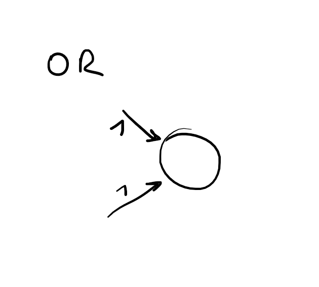
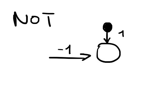
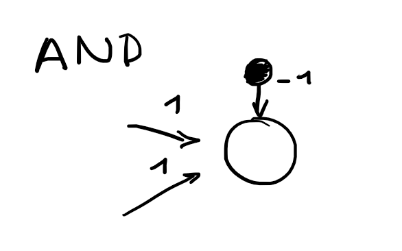
Activation function:

$g(x)=\left\{\begin{array}{ll}1 & \text { if } x \geq 1, \\0 & \text { otherwise }\end{array}\right.$

Boolean functions explained for $g(x)$

in depth

b) Describe the properties of DFIDS and DFS

Depth-first search DFS

Fronier as stack.

Much faster than BFS if solutions are dense.

completeness No - only with explored set and in finite spaces.

time complexity $O(b^m)$ - Terrible results if $m \geq d$ .

space complexity $O(bm)$ - backtracking variant: store one successor node at a time

solution optimality No

Depth-limited search DLS

DFS limited with $\ell$ - returns a $\text{cutoff}$ subtree/subgraph.

Pseudocode

function DEPTH-LIMITED-SEARCH(problem, limit) returns a solution, or failure/cutoff
return RECURSIVE-DLS(MAKE-NODE(problem.INITIAL-STATE), problem, limit)function RECURSIVE-DLS(node, problem, limit) returns a solution, or failure/cutoff
if problem.GOAL-TEST(node.STATE) then return SOLUTION(node)
else if limit = 0 then return cutoff
else
cutoff occurred? ← false
for each action in problem.ACTIONS(node.STATE) do
child ← CHILD-NODE(problem, node, action)
result ← RECURSIVE-DLS(child, problem, limit − 1)
if result = cutoff then cutoff occurred? ← true
else if result != failure then return result
if cutoff occurred? then return cutoff else return failure

completeness No - May not terminate (even for finite search space)

time complexity $O(b^\ell)$

space complexity $O(b\ell )$

solution optimality No

Iterative deepening search IDS

Iteratively increasing $\ell$ in DLS to gain completeness.

Pseudocode

function ITERATIVE-DEEPENING-SEARCH(problem) returns a solution, or failure
for depth = 0 to ∞ do
result ← DEPTH-LIMITED-SEARCH(problem, depth)
if result 6= cutoff then return result

completeness Yes

time complexity $O(b^d)$

in depth
Only $\frac{b}{b-1}$ times more inefficient than BFS therefore $O(b^d)$
IDS(d)=∑i=0dDFS(i)=∑i=0d(∑j=0ibj)=∑i=0dbd+1−1b−1⩽∑i=0dbd+1b−1=bb−1⋅∑i=0dbi=bb−1⋅bd+1−1b−1=bb−1⋅(bb−1⋅bd)=O(bd)IDS(d) = \sum_{i=0}^{d} DFS(i)=\sum_{i=0}^{d} \big( \sum_{j=0}^{i} b^j \big) = \\\sum_{i=0}^{d} \frac{b^{d+1}-1}{b-1} \leqslant \sum_{i=0}^{d} \frac{b^{d+1}}{b-1} = \frac{b}{b-1} \cdot \sum_{i=0}^{d} b^i = \frac{b}{b-1} \cdot \frac{b^{d+1}-1}{b-1} = \\ \frac{b}{b-1} \cdot (\frac{b}{b-1} \cdot b^d) = O(b^d)IDS(d)=i=0∑dDFS(i)=i=0∑d(j=0∑ibj)=i=0∑db−1bd+1−1⩽i=0∑db−1bd+1=b−1b⋅i=0∑dbi=b−1b⋅b−1bd+1−1=b−1b⋅(b−1b⋅bd)=O(bd)

space complexity $O(bd)$

in depth
The total number of nodes generated in the worst case is:
$(d)b +(d-1)b+...+(1)b=O(db)$
Most of the nodes are in the bottom level, so it does not matter much that the upper levels are generated multiple times. In IDS, the nodes on the bottom level (depth $d$ ) are generated once, those on the next-to-bottom level are generated twice, and so on, up to the children of the root, which are generated $d$ times.
Therefore asymptotically the same as DFS.

solution optimality yes, if step cost ≥ 1

c) Name the 4 components of an agents task description.

PEAS: Task description of Agents. ie. Autonomous taxi

Performance measure safety, destination, profits, legality, comfort, . . .

Environment streets/freeways, traffic, pedestrians, weather, . . .

Actuators steering, accelerator, brake, horn, speaker/display, . . .

Sensors video, accelerometers, gauges, engine sensors, keyboard, GPS, . . .

d) What is deep learning, when does it work well, where are its shortcomings?

Deep Learning

Deep learning: Hierarchical structure learning - Artificial neural network with many layers.

Feature extraction and learning (un)supervised

Problem: requires lots of data

Applications of Neural Networks
- Prediction of stock developments
- Prediction of air pollution (e.g., ozone concentration)
- (better than physical/chemical, statistical models)
- Prediction of electric power prizes
- Desulfurization in steel making
- Pattern recognition (e.g., handwriting)
- Face recognition
- Speech recognition
- Handwritten Digit Recognition (OCR)

Advantages and Disadvantages of Neural Networks

Pros

Less need for determining relevant input factors

Inherent parallelism

Easier to develop than statistical methods

Capability to learn and improve

Quite good for complex pattern recognition tasks

Usable for "unstructured" and "difficult" input (e.g., images)

Fault tolerance

Cons

Choice of parameters (layers, units) requires skill

Requires sufficient training material

Resulting hypotheses cannot be understood easily

Knowledge implicit (subsymbolic representation)

Verification, behavior prediction difficult (if not impossible)

Challenges

Interpretability

Explainability

Trustworthiness

Robustness (adversarial examples)

Combining symbolic and subsymbolic approaches

e) Which functions can be represented with single and multi-layer perceptrons?

No hidden layers all linearly seperable functions

One hidden layer all continuous function, can be as precise as one wants

Two hidden layers all functions

Single-layer feed-forward neural networks (Perceptrons)

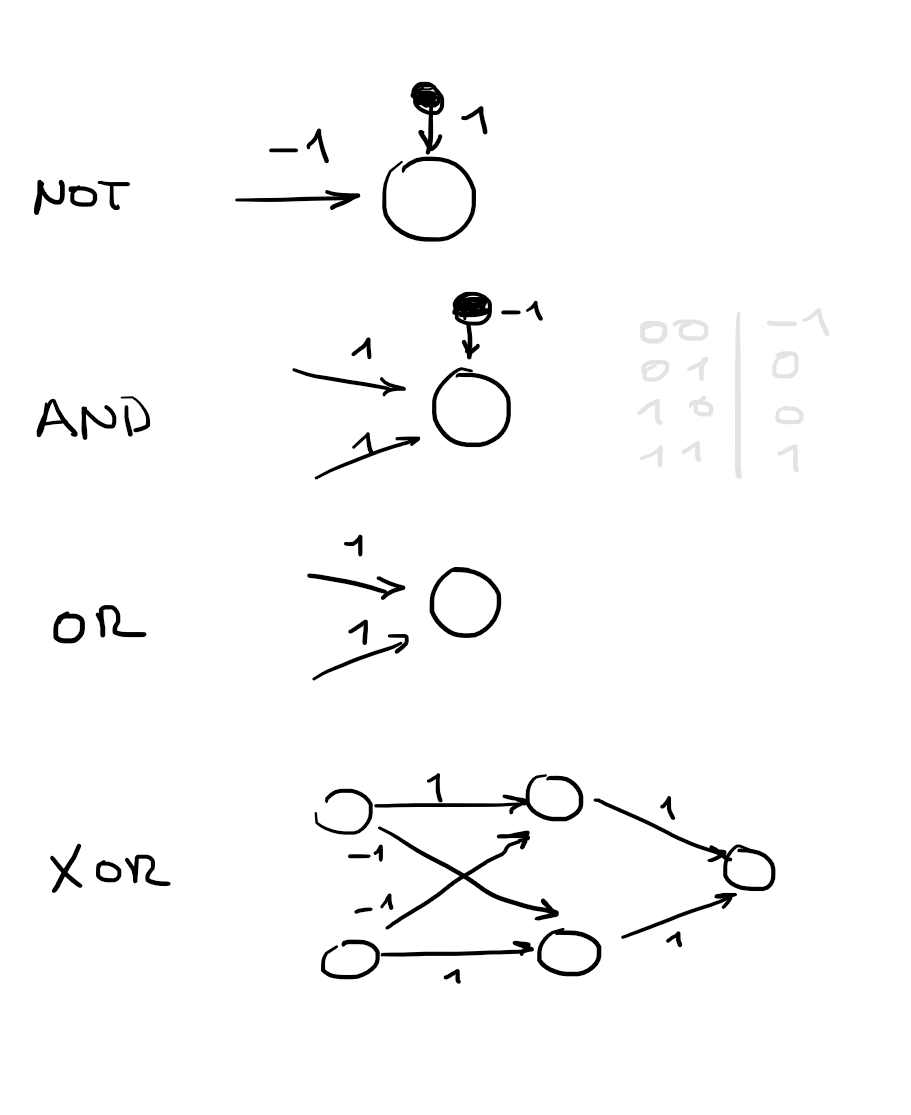
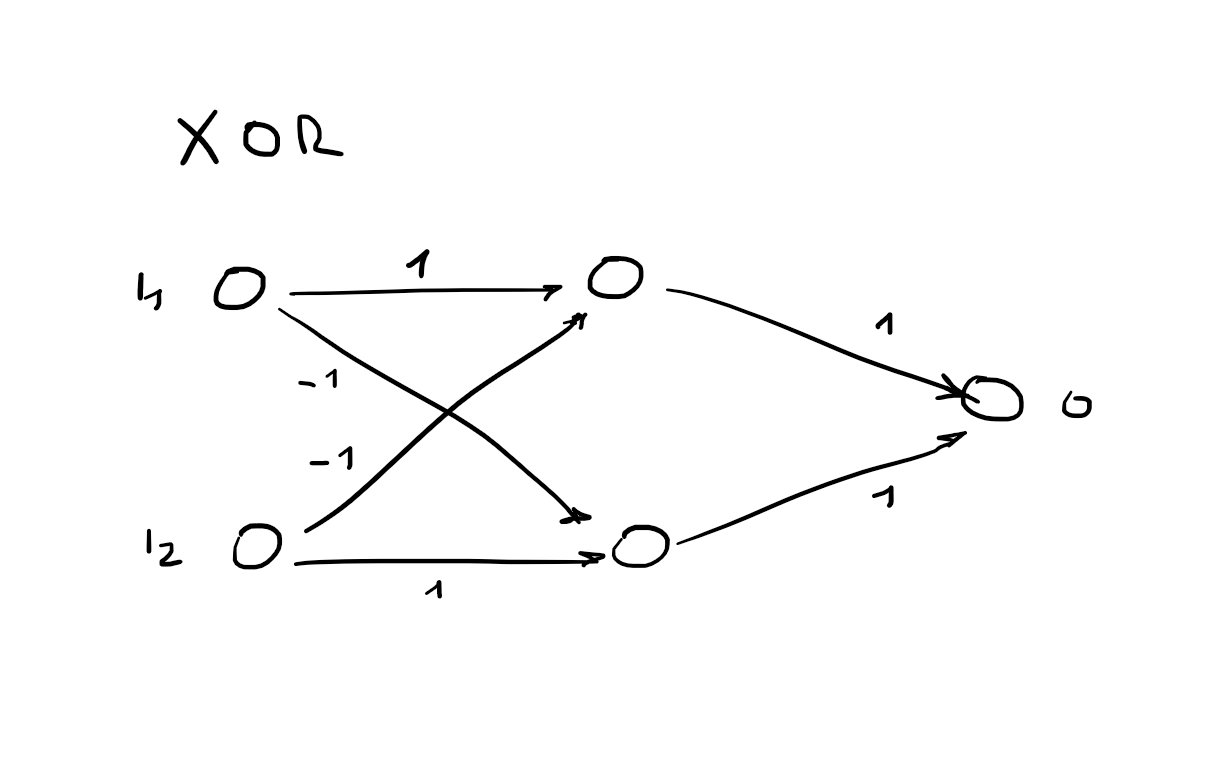
No hidden layers: Always represents a linear separator in the input space - therefore can not represent the XOR function.

Multilayer feed-forward neural networks

With a single, sufficiently large hidden layer (2 layers in total), it is possible to represent any continuous function of the inputs with arbitrary accuracy.

in depth
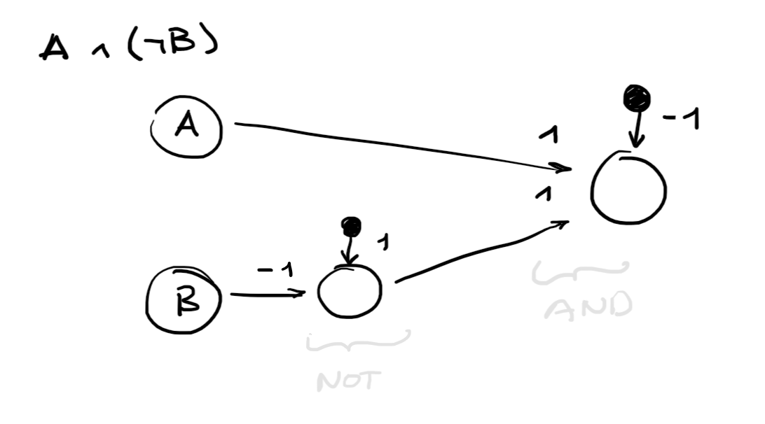
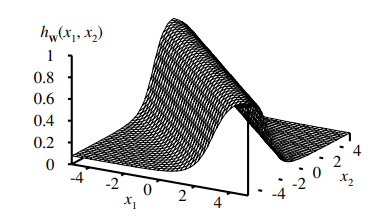
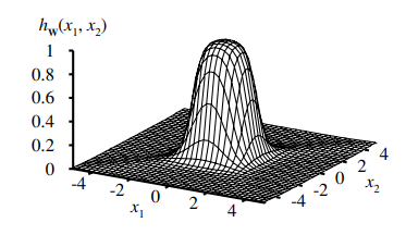
Above we see a nested non-linear function as the solution to the output.
With the sigmoid function as $g$ and a hidden layer, each output unit computes a soft-thresholded linear combination of several sigmoid functions.
For example, by adding two opposite-facing soft threshold functions and thresholding the result, we can obtain a "ridge" function.
Combining two such ridges at right angles to each other (i.e., combining the outputs from four hidden units), we obtain a "bump".
With more hidden units, we can produce more bumps of different sizes in more places.

With two hidden layers, even discontinuous functions can be represented.

f) Prove or contradict the following

$h(n)$ is consistent for all consistent heuristics $h_1, h_2$ if: $h(n) := \max\{h_1(n), h_2(n)\}$

Consistency

For all neighbours $n'$ of $n$ :

$h(n) \leq c\left(n, a, n^{\prime}\right)+h\left(n^{\prime}\right)$

This also implies admissibility and that $f$ is non decreasing along every path
$\begin{aligned}f\left(n^{\prime}\right) &=g\left(n^{\prime}\right)+h\left(n^{\prime}\right) \\&=g(n)+c\left(n, a, n^{\prime}\right)+h\left(n^{\prime}\right) \\& \geq g(n)+h(n)=f(n)\end{aligned}$
$f(n') \geq f(n)$

Proof

$h(n) = \max\{h_1(n), h_2(n)\}$

We know that $h_1$ and $h_2$ are consistent and therefore:

$h_1(n) \leq c\left(n, a, n^{\prime}\right)+h_1\left(n^{\prime}\right)$

$h_2(n) \leq c\left(n, a, n^{\prime}\right)+h_2\left(n^{\prime}\right)$

This means that:

$\begin{aligned}h(n) &=\max\{h_1(n), h_2(n)\}\\& \leq \max\{c(n, a, n^{\prime})+h_1(n^{\prime}), h_2(n) \leq c(n, a, n^{\prime})+h_2(n^{\prime})\}\\& \leq \underbrace{\max\{h_1(n^{\prime}), h_2 (n^{\prime})\}}_{h(n)}+c(n, a, n^{\prime}) \end{aligned}$

Which proves the consistency of $h(n)$ .

g) Describe the working principle of Hill Climbing. What solution are generated when can't solutions be found?

We have 2 local variables: current and neighbour that get chosen randomly in the beginning. (random-restart-hill-climbing).

while(true){
neighbour := highest valued neighbour
if(neigbour.value ≤ current.value) return current.state
else current := neighbour
}

We pick the neighbour with the highest value until there are no higher values left - then we can't climb anymore. Then we return the highest found state.

We can get stuck in local maxima but can escape shoulders.

Part 2)

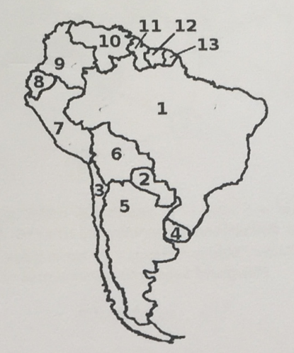
a) Three-colorability problem CSP → Constriant Graph

Variables $\{1,2,3,4,5,6,7,8,9,10,11,12,13\}$

Domains $D_{i}=\{\text { red, green, blue }\}, 1 \leq i \leq 3$

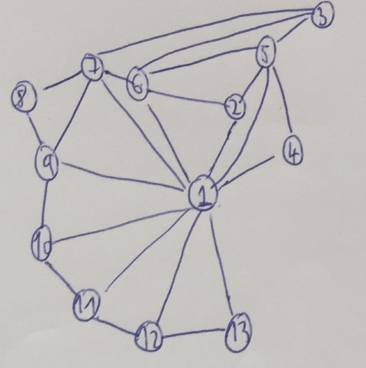
Constraints Adjacent states shall have different colors.

Because we only have binary constrains we can construct the graph as follows:

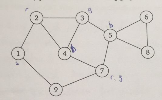
b) Three-colorability problem

Same variables, domains, constraints as before.

Explaination
Different general-purpose methods help improving the performance of the backtracking search.
Variable ordering: fail first
Choose variable with Minimum remaining (legal) values MRV .
Alternatively (as a tie breaker) choose variable that occurs the most often in constraints - degree heuristic .
Value ordering: fail last
least-constraining-value - Choose value that has the least constraints in child nodes

Least-constraining-value heuristic

Partial assignment: $3$ = green, $4$ = blue — which value would $5$ get?

The value $\text{blue}$ would be the least constraining for all neighbours.

Minimum-remaining-values heuristic

Partial assignment: $1$ = blue, $2$ = red, $3$ = green

The variable $4$ has the minimum remaining values in its domains (only one).

Degree heuristic

Which variable would be assigned first?

The variable $5$ has the most neighbours.

c) Explain Backtracking Search for CSPs - why isn't it efficient?

CSPs as standard search problems

If we do not consider commutativity we have $n!d^n$ leafs else we have $d^n$ leafs.

The order of the assignments has no effect on the outcome. - Choosing a single variable variable in each tree level.

Backtracking search algorithm

Uninformed search algorithm (not effective for large trees).

Depth-first search:

chooses values for one unassigned variable at a time - does not matter which one because of commutativity.

tries all values in the domain of that variable

backtracks when a variable has no legal values left to assign.

Because its ineffective we use heuristics / General-purpose methods for backtracking search.

d) Planning: What 3 problems occur in reasoning about actions?

Reasoning about the results of actions

frame problem ... what are things that stay unchanged after action?

ramification problem ... implicit effects (if person is in car, they both move)

qualification problem ... what are preconditions for actions? correct conceptualisation

e) Formalizing in STRIPS an action syntax

$Install$ gets a requested action from a trusted source server and then installs it on the target server.

Predicates:

$\text{Program}(x)$ $x$ is a program

$\text{Server}(x)$ $x$ is a server

$\text{Trusted}(x)$ $x$ is trusted

$\text{Requested}(x)$ $x$ is requested

$\text{Available}(x,y)$ $x$ is only available on $y$

$\operatorname{Action}(Install(p, ss, ts),$

$\text{PRECOND: } \text{Program}(p) \wedge \text{Server}(ss) \wedge \text{Server}(ts) \wedge \text{Trusted}(ss) \wedge \text{Requested}(p) \wedge \text{Available}(p,ss)$

$\text {EFFECT:} ~\neg\text{Requested}(p) \wedge \text{Available}(p,ts)~~)$

f) Describe the node types in decision networks

= influence diagrams.

General framework for rational decisions. Return the action with highest utility.

Decision networks are an extension of Bayesian networks.

Presents:

current state

possible actions

resulting state from actions

utility of each state

Node types:

Chance nodes (ovals) Random variables, uncertainty - Bayes Network

Decision nodes (rectangles) Decision maker has choice of action

Utility nodes (diamonds) Utility function