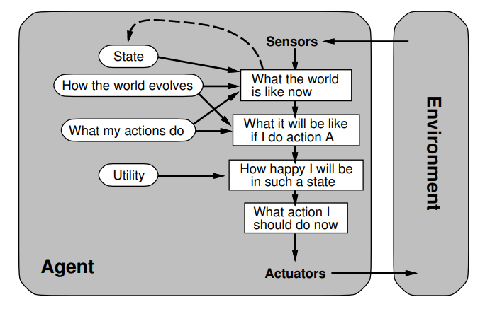
perceptron hard threshhold
g(x)={10 if x≥0 otherwise
sigmoid perceptron logistic function
g(x)=1+e−x1
Deep learning
Hierarchical structure learning: NNs with many layers
Feature extraction and learning (un)supervised
Problem: requires lots of data
Push for hardware (GPUs, designated chips): “Data-Driven” vs. “Model-Driven” computing
d) Multiple choice
1. Local beam search amounts to a locally confined run of
k
random-restart searches. ✅
Idea
keep
k
states instead of just
1
Not the same as running
k
searches in parallel: Searches that find good states recruit other searches to join them - choose top
k
of all their successors
Problem
often, all
k
states end up on same local hill
Solution
choose
k
successors randomly, biased towards good ones
2. Neural networks are generally bad in object recognition. ❌
No - they are particularly good at it.
3. A rational agent does not necessarily always select the best possible action. ✅
Being rational does not mean being:
omniscient (knowing everything) percepts may lack relevant information
clairvoyant (seeing into the future) predictions are not always accurate
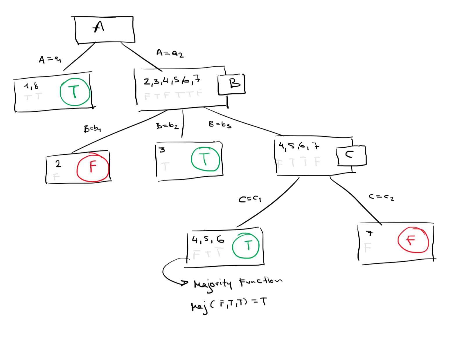
Construct a decision tree from the given data, using the algorithm from the lecture. The next attribute is always chosen
according to the predetermined order:A,B,C
. Which special case occurs? How does the algorithm deal with it?
We have a predefined order, therefore we do not have to calculate the importance of each attribute individually.
The domains of these attributes:
DA={a1,a2}
DB={b1,b2,b3}
DC={c1,c2}
/*
- examples: (x, y) pairs
- attributes: attributes of values x_1, x_2, ... x_n in x in example
- classification: y_j = true / false
*/function DTL(examples, attributes, parent_examples) returns a decision tree
if examples is empty then return MAJORITY(parent_examples.classifications)
else if all examples have the same classification then return the classification
else if attributes is empty then return MAJORITY(examples.classification)
else
A = empty
for each Attribute A' do
A ← maxImportance(A, A', examples)tree ← a new decision tree with root test Afor each (value v of A) do //all possible values from domain of A
exs ← {e : e ∈ examples | e.A = v} //all examples where this value occured
subtree ← DTL(exs, attributes\{A}, examples) //recursive call
add a new branch to tree with label "A = v" and subtree subtreereturn tree
The algorithm is recursive, every sub tree is an independent problem with fewer examples and one less attribute.
The returned tree is not identical to the correct function / tree
f
. It is a hypothesis
h
based on examples.
in depth explaination
no examples left
then it means that there is no example with this combination of values → We return a default value: the majority
function on examples in the parents.
Remaining examples are all positive or negative
we are done
no attributes left but both positive and negative examples
These examples have the same description but different classifications, we return the
plurality-classification
(Reasons: noise in data, non determinism)
some positive or negative examples
choose the most important attribute to split and repeat this process for subtree
In this special case using this predefined order: we have
no attributes left but both positive and negative examples
.
Reason: These examples have the same description but different classifications, we return the
plurality-classification
(Reasons: noise in data, non determinism)
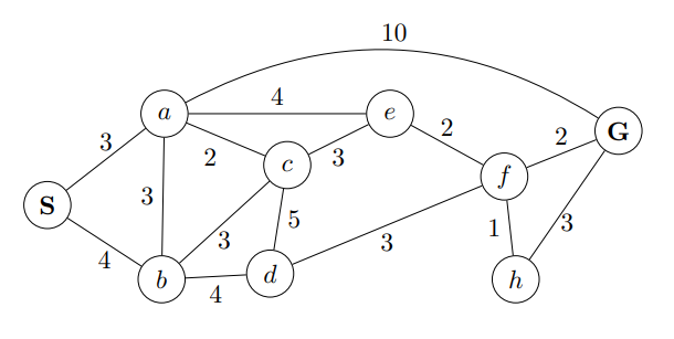
StepPriority queue before stepPath after stepCost0S(10)S01a(10),b(12)S→a32b(12),c(10),e(9),G(13)S→a→e73b(12),c(10),f(11),G(13)S→a→c54b(12),d(13),f(11),G(13)S→a→e→f95b(12),d(13),h(10),G(11)S→a→e→f→h106b(12),d(13),G(11)S→a→e→f→G11\begin{array}{|c|l|l|c|} \hline \text { Step } & \text { Priority queue before step } & \text { Path after step } & \text { Cost } \\\hline \hline 0 & S(10) & S & 0 \\\hline 1 & a(10), b(12) & S \rightarrow a & 3 \\\hline 2 & \textcolor{grey}{ b(12)}, c(10), e(9), G(13) & S \rarr a \rarr e & 7 \\\hline 3 & \textcolor{grey}{ b(12)}, \textcolor{grey}{c(10)}, f(11), \textcolor{grey}{G(13)} & S \rarr a \rarr c & 5 \\\hline 4 & \textcolor{grey}{ b(12)}, d(13), \textcolor{grey}{ f(11)}, \textcolor{grey}{G(13)} & S \rarr a \rarr e \rarr f & 9 \\\hline 5 & \textcolor{grey}{ b(12)}, \textcolor{grey}{ d(13)}, h(10),G(11) & S \rarr a \rarr e \rarr f \rarr h& 10 \\\hline 6 & \textcolor{grey}{ b(12)}, \textcolor{grey}{d(13)},\textcolor{grey}{ G(11)} & S \rarr a \rarr e \rarr f \rarr G& 11 \\\hline\end{array}Step0123456Priority queue before stepS(10)a(10),b(12)b(12),c(10),e(9),G(13)b(12),c(10),f(11),G(13)b(12),d(13),f(11),G(13)b(12),d(13),h(10),G(11)b(12),d(13),G(11)Path after stepSS→aS→a→eS→a→cS→a→e→fS→a→e→f→hS→a→e→f→GCost037591011
If I marked it grey, that means its from another step.
Were using a graph search algorithm with an explored set.
This is the explored set (seen in the correct order):
explored={S,a,e,c,f,g}
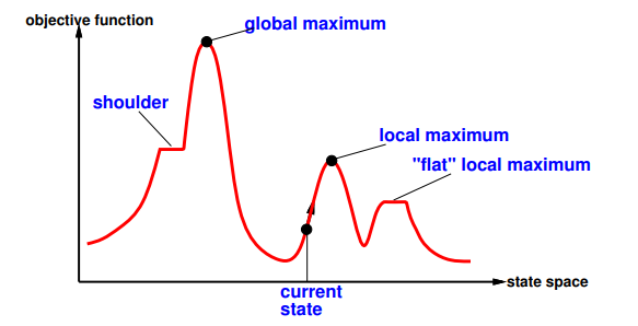
g) Describe how hill climbing functions. Which problem can occur? Whats the solution to it?
Also called "hill-climbing":
+
escaping shoulders
−
getting stuck in loop at local maximum
Solution: Random-restart hill climbing: restart after step limit overcomes local maxima
Pseudocode
function HILL-CLIMBING(problem) returns a state that is a local maximum
inputs: problem // a problem
local variables:
current, // a node
neighbor // a node
current ← MAKE-NODE(INITIAL-STATE[problem])
loop do
neighbor ← a highest-valued successor of current
if VALUE[neighbor] ≤ VALUE[current] then return STATE[current]
current ← neighbor
h) DFS vs. IDS - are they optimal with infinite branching factors?
They still must terminate at some point even with infinite branches, since they use a stack as their frontier-set data-structure.
They explore the tree in its full depth first before continuing with its breadth.
3) Depth-first search DFS
Fronier as stack.
Much faster than BFS if solutions are dense.
Backtracking variant: store one successor node at a time - generate child node with
Δ
change.
completeness
No - only complete with explored set and in finite spaces.
time complexityO(bm)
- Terrible results if
m≥d
.
space complexityO(bm)
solution optimality
No
4) Depth-limited search DLS
DFS limited with
ℓ
- returns a
cutoff
subtree/subgraph.
Pseudocode
function DEPTH-LIMITED-SEARCH(problem, limit) returns a solution, or failure/cutoff
return RECURSIVE-DLS(MAKE-NODE(problem.INITIAL-STATE), problem, limit)function RECURSIVE-DLS(node, problem, limit) returns a solution, or failure/cutoff
if problem.GOAL-TEST(node.STATE) then return SOLUTION(node)
else if limit = 0 then return cutoff
else
cutoff occurred? ← false
for each action in problem.ACTIONS(node.STATE) do
child ← CHILD-NODE(problem, node, action)
result ← RECURSIVE-DLS(child, problem, limit − 1)
if result = cutoff then cutoff occurred? ← true
else if result != failure then return result
if cutoff occurred? then return cutoff else return failure
completeness
No - May not terminate (even for finite search space)
time complexityO(bℓ)
space complexityO(bℓ)
solution optimality
No
5) Iterative deepening search IDS
Iteratively increasing
ℓ
in DLS to gain completeness.
Pseudocode
function ITERATIVE-DEEPENING-SEARCH(problem) returns a solution, or failure
for depth = 0 to ∞ do
result ← DEPTH-LIMITED-SEARCH(problem, depth)
if result 6= cutoff then return result
completeness
Yes
time complexityO(bd)
in depth
Only
b−1b
times more inefficient than BFS therefore
O(bd)
The total number of nodes generated in the worst case is:
(d)b+(d−1)b+...+(1)b=O(db)
Most of the nodes are in the bottom level, so it does not matter much that the upper levels are generated multiple times. In
IDS, the nodes on the bottom level (depth
d
) are generated once, those on the next-to-bottom level are generated twice, and so on, up to the children of the root,
which are generated
d
times.
Therefore asymptotically the same as DFS.
solution optimality
Yes, if step cost ≥ 1
Part 2
a) Cryptographic puzzle as a CSP
  E G G
+ O I L
-------
M A Y O
Defined as a constraint satisfaction problem:
X={E,G,O,I,L,A,Y,X1,X2,X3}
D={0,1,2,3,4,5,6,7,8,9}
Constraints:
Each letter stands for a different digit:
Alldiff(E,G,O,I,L,A,Y)
The
X1,X2,X3
variables stand for the digit that gets carried over into the next column by the addition. Therefore
X1
stands for
10
in our unknown numeric system,
X2
stands for
100
,
X3
stands for
1000
.
b) 3-color-problem and backtracking-search heuristics
Least constraining value
Partial assignment:
1=green,2=red
Question: Which value would be assigned to the variable
3
by the least-constraining-value heuristic?
Answer:
3=red
Minimum remaining values
Partial assignment:
2=blue, 5=red ,7=green
Question: Which variable would be assigned next using the minimum-remaining-values heuristic?
Answer
4
Degree heuristic
Question: Which variable would be assigned a value from its domain first by the degree heuristic?
Answer:
4
Explanation
Variable ordering: fail first
Minimum remaining (legal) values MRV
degree heuristic - (used as a tie breaker), variable that occurs the most often in constraints
Value ordering: fail last
least-constraining-value - a value that rules out the fewest choices for the neighbouring variables in the constraint graph.
c) Multiple Choice
1. A CSP can only contain binary constraints ❌
Backtracking search algorithm
Depth-first search with single-variable assignments:
chooses values for one unassigned variable at a time - does not matter which one because of commutativity.
tries all values in the domain of that variable
backtracks when a variable has no legal values left to assign.
2. The backtracking search is an uninformed search algorithm. ✅
3. The axiom of continuity is:
A≻B≻C⇒∃p[p,A;1−p,B]∼C
❌
The right answer would be
A≻B≻C⇒∃p[p,A;1−p,C]∼B
d) Axiom of monotonicity from utility theory
Monotonicity
Agent prefers a higher probability of the state that it prefers.
A≻B⇒(p>q⇔[p,A;1−p,B]≻[q,A;1−q,B])
e) Multiple Choice
1. Classical planning environments are static ✅
Classical Planning Environments
Used in classical planning:
fully observable
deterministic, finite
static (change happens only when the agent acts)
discrete in time, actions, objects, and effects
2.
∃xMeets(x,bob)
is syntactically correct in STRIPS ❌
No, STRIPS does not support quantors.
3. Unlike STRIPS, ADL supports equality ✅
4. In partial order planning, the constraint
A≺B
means that
A
must be executed immediately before
B
❌
It means that
A
must be executed some time before
B
.