Search Problem Definition

Real World → Search problem → Search Algorithm

Solution

A solution is a sequence of actions leading from the initial state to a goal state.

• Example

  We are on a holiday in Romania, Arad. Our flight leaves tomorrow from Bucharest.

  1. initial state

     starting_state = "at Arad"

  2. successor function

     S(prevState)={<prevState -> action, nextState>, ...}

     S(Arad)={<Arad -> gotoZerind, Zerind>, ...}

  3. goal test

     explicit:x == "at Bucharest"

     implicit:hasAirport(x, "Bucharest")

  4. path cost (additive)

     sum of distances, number of actions executed,$\dots$

     c(x, a, y)is the step cost, assumed to be ≥ 0

Goal testing

• at expansion

• at generation → better performance, only storing necessary nodes

Tree-Search algorithm TS

Offline, simulated exploration of state space.

The frontier / open list set contains all child nodes that can be expanded.

• Pseudocode

  function TREE-SEARCH(problem) returns a solution, or failure
  initialize the frontier using the initial state of problem
  loop do
  if the frontier is empty then return failure
  choose a leaf node and remove it from the frontier
  if the node contains a goal state then return the corresponding solution
  expand the chosen node, adding the resulting nodes to the frontier

Graph-Search algorithm GS

Same as tree search but also stores all visited nodes in an explored set / closed list of already considered states to prevent endless looping.

Can be exponentially more efficient than tree search.

• Pseudocode

  function GRAPH-SEARCH(problem) returns a solution, or failure
  initialize the frontier using the initial state of problem
  initialize the explored set to be empty
  loop do
  if the frontier is empty then return failure
  choose a leaf node and remove it from the frontier
  if the node contains a goal state then return the corresponding solution
  add the node to the explored set
  expand the chosen node, adding the resulting nodes to the frontier

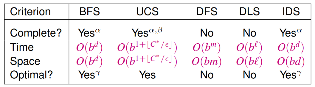
Uninformed search algorithms

completeness always finds existing solutions

space complexity max number of nodes in memory

time complexity max number of nodes generated/expanded.

solution optimality always finds the least-cost solution

$b$ maximum branching factor of search tree

$d$ depth of shallowest solution

$m$ maximum depth (may be $\infin$ )

$\ell$ depth limit

Overview

under the conditions:

$\alpha$- if $b$ is finite

$\beta$- if step costs $\geq \varepsilon$ for positive $\varepsilon$

$\gamma$- optimal with identical step costs

1) Breadth-first search BFS

Frontier as queue.

The space and time complexity is too high.

Here the goal test is done at generation time.

• Pseudocode

  function BREADTH-FIRST-SEARCH(problem) returns a solution, or failure
  node ← a node with STATE = problem.INITIAL-STATE, PATH-COST = 0
  if problem.GOAL-TEST(node.STATE) then return SOLUTION(node)
  frontier ← a FIFO queue with node as the only element
  explored ← an empty set
  loop do
  if EMPTY?(frontier) then return failure
  node ← POP(frontier)
  add node.STATE to explored
  for each action in problem.ACTIONS(node.STATE) do
  child ← CHILD-NODE(problem, node, action)
  if child.STATE is not in explored or frontier then
  if problem.GOAL-TEST(child.STATE) then return SOLUTION(child)
  frontier ← INSERT(child,frontier)

completeness yes, if $b$ is finite

time complexity$O(b^d)$

space complexity$O(b^d)$

solution optimality yes, if step costs ≥ 1

2) Uniform-cost search UCS

Fronier as priority queue ordered by costs.

Here the goal test is done at expansion time.

• Pseudocode

  function UNIFORM-COST-SEARCH(problem) returns a solution, or failure
  node ← a node with STATE = problem.INITIAL-STATE, PATH-COST = 0
  frontier ← a priority queue ordered by PATH-COST, with node as the only element
  explored ← an empty set
  loop do
  if EMPTY?(frontier) then return failure
  node ← POP(frontier)
  if problem.GOAL-TEST(node.STATE) then return SOLUTION(node)
  add node.STATE to explored
  for each action in problem.ACTIONS(node.STATE) do
  child ← CHILD-NODE(problem, node, action)
  if child.STATE is not in explored or frontier then
  frontier ← INSERT(child,frontier)
  else if child.STATE is in frontier with higher PATH-COST then
  replace that frontier node with child

completeness Yes, if step-cost $\geq \varepsilon$ and $b$ is finite

time complexity$O(b^{\lfloor C^*/ \varepsilon \rfloor +1})$

space complexity$O(b^{\lfloor C^*/ \varepsilon \rfloor +1})$

solution optimality Yes, if goal-tested at expansion.

3) Depth-first search DFS

Fronier as stack.

Much faster than BFS if solutions are dense.

Backtracking variant: store one successor node at a time - generate child node with $\Delta$ change.

completeness No - only complete with explored-set (graph search) and in finite spaces.

time complexity$O(b^m)$ - Terrible results if $m \geq d$ .

space complexity$O(bm)$

solution optimality No

4) Depth-limited search DLS

DFS limited with $\ell$ - returns a $\text{cutoff}$ subtree/subgraph.

• Pseudocode

  function DEPTH-LIMITED-SEARCH(problem, limit) returns a solution, or failure/cutoff
  return RECURSIVE-DLS(MAKE-NODE(problem.INITIAL-STATE), problem, limit)function RECURSIVE-DLS(node, problem, limit) returns a solution, or failure/cutoff
  if problem.GOAL-TEST(node.STATE) then return SOLUTION(node)
  else if limit = 0 then return cutoff
  else
  cutoff occurred? ← false
  for each action in problem.ACTIONS(node.STATE) do
  child ← CHILD-NODE(problem, node, action)
  result ← RECURSIVE-DLS(child, problem, limit − 1)
  if result = cutoff then cutoff occurred? ← true
  else if result != failure then return result
  if cutoff occurred? then return cutoff else return failure

completeness No - May not terminate (even for finite search space)

time complexity$O(b^\ell)$

space complexity$O(b\ell )$

solution optimality No

5) Iterative deepening search IDS

Iteratively increasing $\ell$ in DLS to gain completeness.

• Pseudocode

  function ITERATIVE-DEEPENING-SEARCH(problem) returns a solution, or failure
  for depth = 0 to ∞ do
  result ← DEPTH-LIMITED-SEARCH(problem, depth)
  if result 6= cutoff then return result

completeness Yes

time complexity$O(b^d)$

space complexity$O(bd)$

solution optimality Yes, if step cost ≥ 1

In general IDS is very attractive and prefered when the search space is large and the depth of the solution is unknown.

It is usually only a little more expensive than BFS.