All exam questions so far + answers

Agents

• Environments that agents can be situated in

  fully observable vs. partly observable

  whether sensors can detect all relevant properties

  single-agent vs. multi-agent

  single agent, or multiple with cooperation, competition

  deterministic vs. stochastic

  whether the next state can be determined by current state + the performed action or is fully independent and can't be foreseen (multiple possible following states) - and we know the probabilities

  episodic vs. sequential

  Episodic: the choice of action only depends on the current episode - percept history divided into independent episodes.

  Sequential: storing entire history (accessing memories lowers performance)

  static vs. dynamic vs. semi-dynamic

  Static: world does not change during the reasoning / processing time of the agent (waits for agents response)

  Semi-dynamic: environment is static, but performance score decreases while processing time.

  discrete vs. continuous

  property values of the world

  known vs. unknown

  state of knowledge about the "laws of physics" of the environment

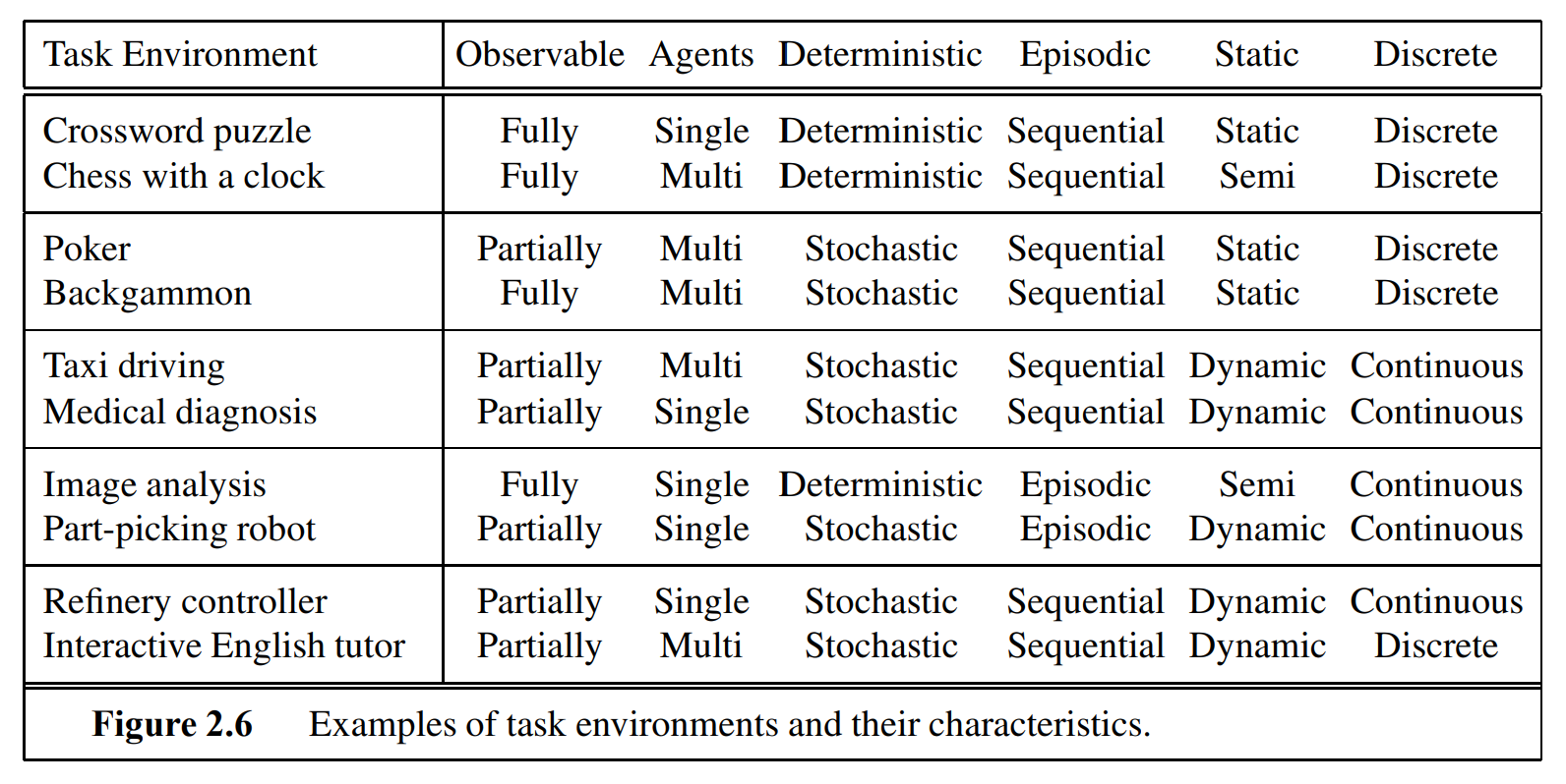
  • Example

    A game of poker is in a discrete environment.

    

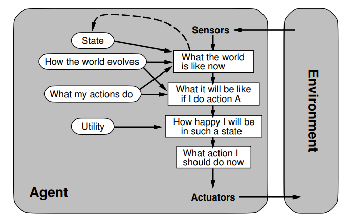
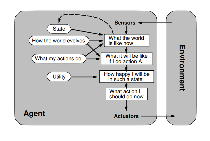
• Name the 4 components of an agents task description

  Task description of Agents. ie: Autonomous car

  Performance measure safety, destination, profits, legality, comfort, . . .

  Environment streets/freeways, traffic, pedestrians, weather, . . .

  Actuators steering, accelerator, brake, horn, speaker/display, . . .

  Sensors video, accelerometers, gauges, engine sensors, keyboard, GPS, . . .

• Rational agent

  Chooses action that maximizes performance measure outuput for any percept sequence.

  Decisions based on evidence:

  • percept history

  • built-in knowledge of the environment (if the environment is known)- ie. fundamental knowledge laws like physics

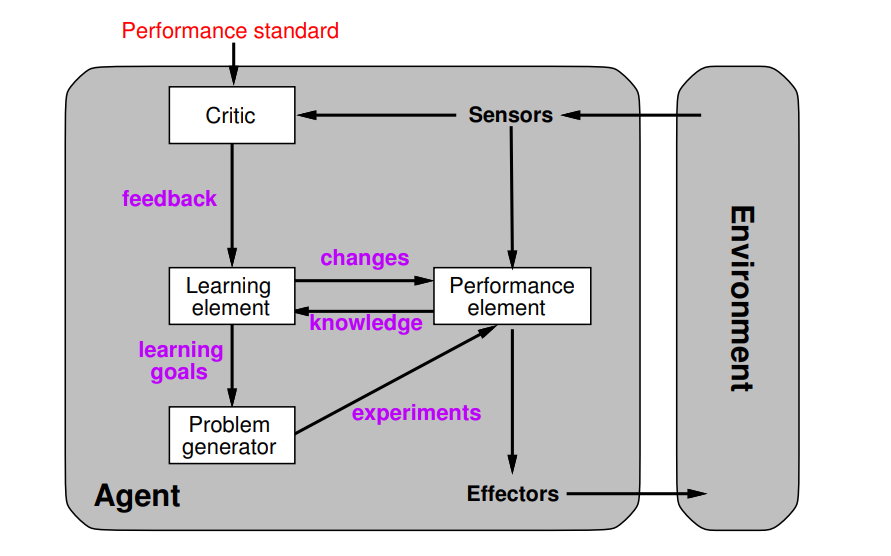
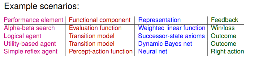
• Agent types

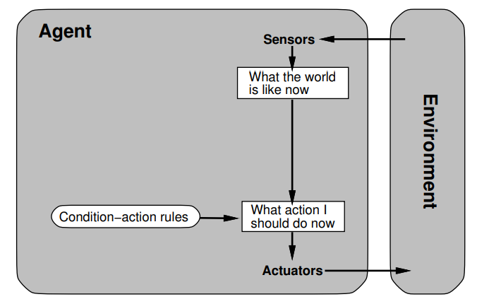
  • Simple reflex agents

    • No memory (percept sequences)

    • no internal states

    • Possible non-termination

    • Only suitable for very specific tasks

    

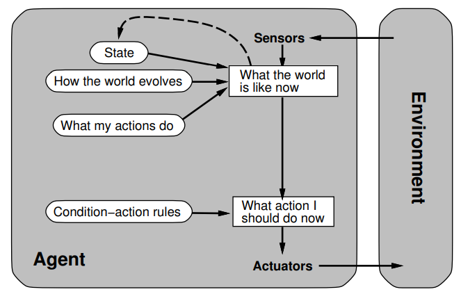
  • Model-based reflex agent

    • memory

    • internal states of the world

    • model of environment and changes in it

    • can reason about unobservable parts

    • can deal with uncertainty

    • has implicit goals

    

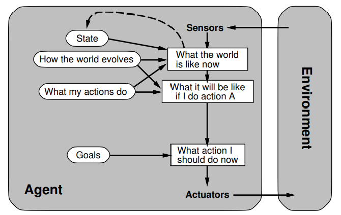
  • Goal-based agents

    • explicit goals

    • explicitly model: the world , goals, actions and their effects

    • Search and planning of action sequences

    • more flexible, better maintainability

    

  • Utility-based agents

    • evaluate goals with utility function

    • use expected utility for decisions

    • resolve conflicting goals - goals are weighted differently, the aim is to optimize a set of values

    

• goal based agent vs. utility based agent

  The goal based agent

  • can not deal with conflicting goals because it does not have a utility function.

  • Does not consider expected utility when planning - just goals, actions, effects.

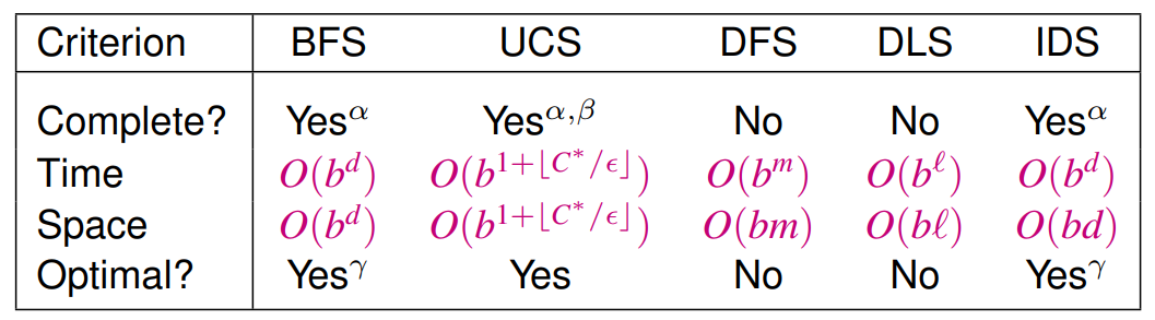
Uninformed search algorithms

• Formal description of a search problem

  Real World → Search problem → Search Algorithm

  We define states, actions, solutions (= selecting a state space) through abstraction.

  Then we turn states into nodes for the search algorithm.

  Solution

  A solution is a sequence of actions leading from the initial state to a goal state.

  1. Initial state

  2. Successor function

  3. Goal test

  4. path cost (additive)

• All algorithms

  • Breadth-first search BFS

    Frontier as queue.

    The space and time complexity is too high.

    Here the goal test is done at generation time.

    • Pseudocode

      function BREADTH-FIRST-SEARCH(problem) returns a solution, or failure
      node ← a node with STATE = problem.INITIAL-STATE, PATH-COST = 0
      if problem.GOAL-TEST(node.STATE) then return SOLUTION(node)
      frontier ← a FIFO queue with node as the only element
      explored ← an empty set
      loop do
      if EMPTY?(frontier) then return failure
      node ← POP(frontier)
      add node.STATE to explored
      for each action in problem.ACTIONS(node.STATE) do
      child ← CHILD-NODE(problem, node, action)
      if child.STATE is not in explored or frontier then
      if problem.GOAL-TEST(child.STATE) then return SOLUTION(child)
      frontier ← INSERT(child,frontier)

    completeness yes, if $b$ is finite

    time complexity$O(b^d)$

    • in depth

      If solution is at depth $d$ and max branching is $b$ :

      ∑i=0dbi=bd+1−1b−1=bb−1⋅bd=O(bd)\sum_{i=0}^{d} b^i = \frac{b^{d+1}-1}{b-1} = \frac{b}{b-1} \cdot b^d = O(b^d)i=0∑d​bi=b−1bd+1−1​=b−1b​⋅bd=O(bd)

      Goal test at generation time: $1 + b + b^2 + b^3 + ... + b^d = O(b^d)$

      Goal test at expansion time: $1 + b + b^2 + b^3 + ... + b^d + \textcolor{pink}{b^{d+1}}= O(b^{d+1})$

    space complexity$O(b^d)$

    solution optimality yes, if step costs are identical

  • Uniform-cost search UCS

    Fronier as priority queue ordered by costs.

    Here the goal test is done at expansion time.

    • Pseudocode

      function UNIFORM-COST-SEARCH(problem) returns a solution, or failure
      node ← a node with STATE = problem.INITIAL-STATE, PATH-COST = 0
      frontier ← a priority queue ordered by PATH-COST, with node as the only element
      explored ← an empty set
      loop do
      if EMPTY?(frontier) then return failure
      node ← POP(frontier)
      if problem.GOAL-TEST(node.STATE) then return SOLUTION(node)
      add node.STATE to explored
      for each action in problem.ACTIONS(node.STATE) do
      child ← CHILD-NODE(problem, node, action)
      if child.STATE is not in explored or frontier then
      frontier ← INSERT(child,frontier)
      else if child.STATE is in frontier with higher PATH-COST then
      replace that frontier node with child

    completeness Yes, if step-cost $\geq \varepsilon$ and $b$ is finite

    time complexity$O(b^{\lfloor C^*/ \varepsilon \rfloor +1})$

    • in depth

      if all step-costs $\geq\varepsilon$

      and $C^*$ is the cost of the optimal solution

      then $d = {\lfloor \frac{ C^* }{ \varepsilon}\rfloor +1}$ and therefore $O(b^{\lfloor C^*/ \varepsilon \rfloor +1})$

      if goal-tested at expansion, not generation - therefore $b^{d+1}$ .

    space complexity$O(b^{\lfloor C^*/ \varepsilon \rfloor +1})$

    solution optimality Yes, if goal-tested at expansion.

  • Depth-first search DFS

    Fronier as stack.

    Much faster than BFS if solutions are dense.

    Backtracking variant: store one successor node at a time - generate child node with $\Delta$ change.

    completeness No - only complete with explored-set and in finite spaces.

    time complexity$O(b^m)$ - Terrible results if $m \geq d$ .

    space complexity$O(bm)$

    solution optimality No

  • Depth-limited search DLS

    DFS limited with $\ell$ - returns a $\text{cutoff}$ subtree/subgraph.

    • Pseudocode

      function DEPTH-LIMITED-SEARCH(problem, limit) returns a solution, or failure/cutoff
      return RECURSIVE-DLS(MAKE-NODE(problem.INITIAL-STATE), problem, limit)function RECURSIVE-DLS(node, problem, limit) returns a solution, or failure/cutoff
      if problem.GOAL-TEST(node.STATE) then return SOLUTION(node)
      else if limit = 0 then return cutoff
      else
      cutoff occurred? ← false
      for each action in problem.ACTIONS(node.STATE) do
      child ← CHILD-NODE(problem, node, action)
      result ← RECURSIVE-DLS(child, problem, limit − 1)
      if result = cutoff then cutoff occurred? ← true
      else if result != failure then return result
      if cutoff occurred? then return cutoff else return failure

    completeness No - May not terminate (even for finite search space)

    time complexity$O(b^\ell)$

    space complexity$O(b\ell )$

    solution optimality No

  • Iterative deepening search IDS

    Iteratively increasing $\ell$ in DLS to gain completeness.

    • Pseudocode

      function ITERATIVE-DEEPENING-SEARCH(problem) returns a solution, or failure
      for depth = 0 to ∞ do
      result ← DEPTH-LIMITED-SEARCH(problem, depth)
      if result 6= cutoff then return result

    completeness Yes - if $b$ is finite

    time complexity$O(b^d)$

    • in depth

      Only $\frac{b}{b-1}$ times more inefficient than BFS therefore $O(b^d)$

      IDS(d)=∑i=0dDFS(i)=∑i=0d(∑j=0ibj)=∑i=0dbd+1−1b−1⩽∑i=0dbd+1b−1=bb−1⋅∑i=0dbi=bb−1⋅bd+1−1b−1=bb−1⋅(bb−1⋅bd)=O(bd)IDS(d) = \sum_{i=0}^{d} DFS(i)=\sum_{i=0}^{d} \big( \sum_{j=0}^{i} b^j \big) = \\\sum_{i=0}^{d} \frac{b^{d+1}-1}{b-1} \leqslant \sum_{i=0}^{d} \frac{b^{d+1}}{b-1} = \frac{b}{b-1} \cdot \sum_{i=0}^{d} b^i = \frac{b}{b-1} \cdot \frac{b^{d+1}-1}{b-1} = \\ \frac{b}{b-1} \cdot (\frac{b}{b-1} \cdot b^d) = O(b^d)IDS(d)=i=0∑d​DFS(i)=i=0∑d​(j=0∑i​bj)=i=0∑d​b−1bd+1−1​⩽i=0∑d​b−1bd+1​=b−1b​⋅i=0∑d​bi=b−1b​⋅b−1bd+1−1​=b−1b​⋅(b−1b​⋅bd)=O(bd)

    space complexity$O(bd)$

    • in depth

      The total number of nodes generated in the worst case is:

      $(d)b +(d-1)b+...+(1)b=O(db)$

      Most of the nodes are in the bottom level, so it does not matter much that the upper levels are generated multiple times. In IDS, the nodes on the bottom level (depth $d$ ) are generated once, those on the next-to-bottom level are generated twice, and so on, up to the children of the root, which are generated $d$ times.

      Therefore asymptotically the same as DFS.

    solution optimality Yes, if step cost are identical

  ---

  • Overview

    

    under the conditions:

    $\alpha$- if $b$ is finite

    $\beta$- if step costs $\geq \varepsilon$ for positive $\varepsilon$

    $\gamma$- optimal with identical step costs

• Does BFS expand as many nodes as DFS?

  No - they have different frontier expansion strategies

  but in some cases this can be true (as it depends on the graph).

  But BFS expands nodes in the same tree level first while DFS expands all children of the same node until there aren't any left.

• Is IDS optimal for limited tree depth?

  No - it is only optimal with with identical step costs.

• Does BFS expand at least as often as it has nodes?

  BFS can goal check:

  • At expansion time - expands as often as it has nodes at most

  • At generation time (more efficient - expands less than it has nodes)

• Is BFS a special case of A* search?

  If we set the heuristic to $h(n) = 0$ for every node and $g(n) = depth(n)$ then A* acts as BFS:

  $f(n) = depth(n)$

  Choosing function with the lowest depth in the tree first.

Informed Search

• consistency: Admissible heuristics have a problem with graph search. Which one is it? How can this problem be solved?

  Implies that $f$ -value is non-decreasing on every path .

  For every node $n$ and its successor $n'$ :

  $h(n) \leq c(n,a,n') + h(n')$

  • consistent $h(n)$ for graph search is optimal

    If $h(n)$ decreases during optimal path to goal it is discarded by graph-search .

    (But in tree search it is not a problem since there is only a single path to the optimal goal).

    Solutions to problem:

    • consistency of $h$ (non decreasing $f$ on every path)

    • additional book-keeping

• Given admissible heuristics $(h_1, h_2, \dots, h_n)$ . Which one is the best?

  The heuristic that dominates the others:

  For two admissible heuristics, we say $h_2$ dominates $h_1$ , if:

  $\forall n: h_2(n) \geq h_1(n)$

  Then $h_2$ is better for search.

• admissibility

  Optimistic, never overestimating, never negative.

  $h(n) \leq f^*(n)$

  $h(n) \geq 0$

  $\forall g$ goals: $h(g)=0$(follows from the above)

• Prove: If the heuristic is consistent and $n'$ is the neighbour of $n$ , then $f(n') \geq f(n)$

  $f(n') = g(n') + h(n')= g(n) + {c(n, a,n') + h(n')}$

  $f(n') = g(n) + \textcolor{pink}{c(n, a,n') + h(n')} \geq g(n) +\textcolor{pink}{ h(n)} = f(n)$(because of consistency)

  $f(n') \geq f(n)$

• Prove: $h(n)$ is consistent for all consistent heuristics $h_1, h_2$ if: $h(n) := \max\{h_1(n), h_2(n)\}$

  $h(n) = \max\{h_1(n), h_2(n)\}$

  We know that $h_1$ and $h_2$ are consistent and therefore:

  $h_1(n) \leq c\left(n, a, n^{\prime}\right)+h_1\left(n^{\prime}\right)$

  $h_2(n) \leq c\left(n, a, n^{\prime}\right)+h_2\left(n^{\prime}\right)$

  This means that:

  $\begin{aligned}h(n) &=\max\{h_1(n), h_2(n)\}\\& \leq \max\{c(n, a, n^{\prime})+h_1(n^{\prime}), h_2(n) \leq c(n, a, n^{\prime})+h_2(n^{\prime})\}\\& \leq \underbrace{\max\{h_1(n^{\prime}), h_2 (n^{\prime})\}}_{h(n)}+c(n, a, n^{\prime}) \end{aligned}$

  Which proves the consistency of $h(n)$ .

Local Search

• local beam search and its advantages / disadvantages

  Idea

  • keep $k$ states instead of just $1$ to start searching from

  • Not running $k$ searches in parallel: Searches that find good states recruit other searches to join them

  • choose top $k$ of all their successors

  Problem

  often, all $k$ states end up on same local hill

  Solution

  choose $k$ successors randomly, biased towards good ones

• Is local beam search a modification of the generic algorithm with cross-over?

  yes - the genetic algorithm = stochastic local beam search + successors from pairs of states

• hill climbing algorithm - how do we deal with its weaknesses?

  Advantage: able of escaping shoulders

  Disadvantage: getting stuck in loop at local maximum

  Solution: Random-restart hill climbing = restart after step

Decision Trees

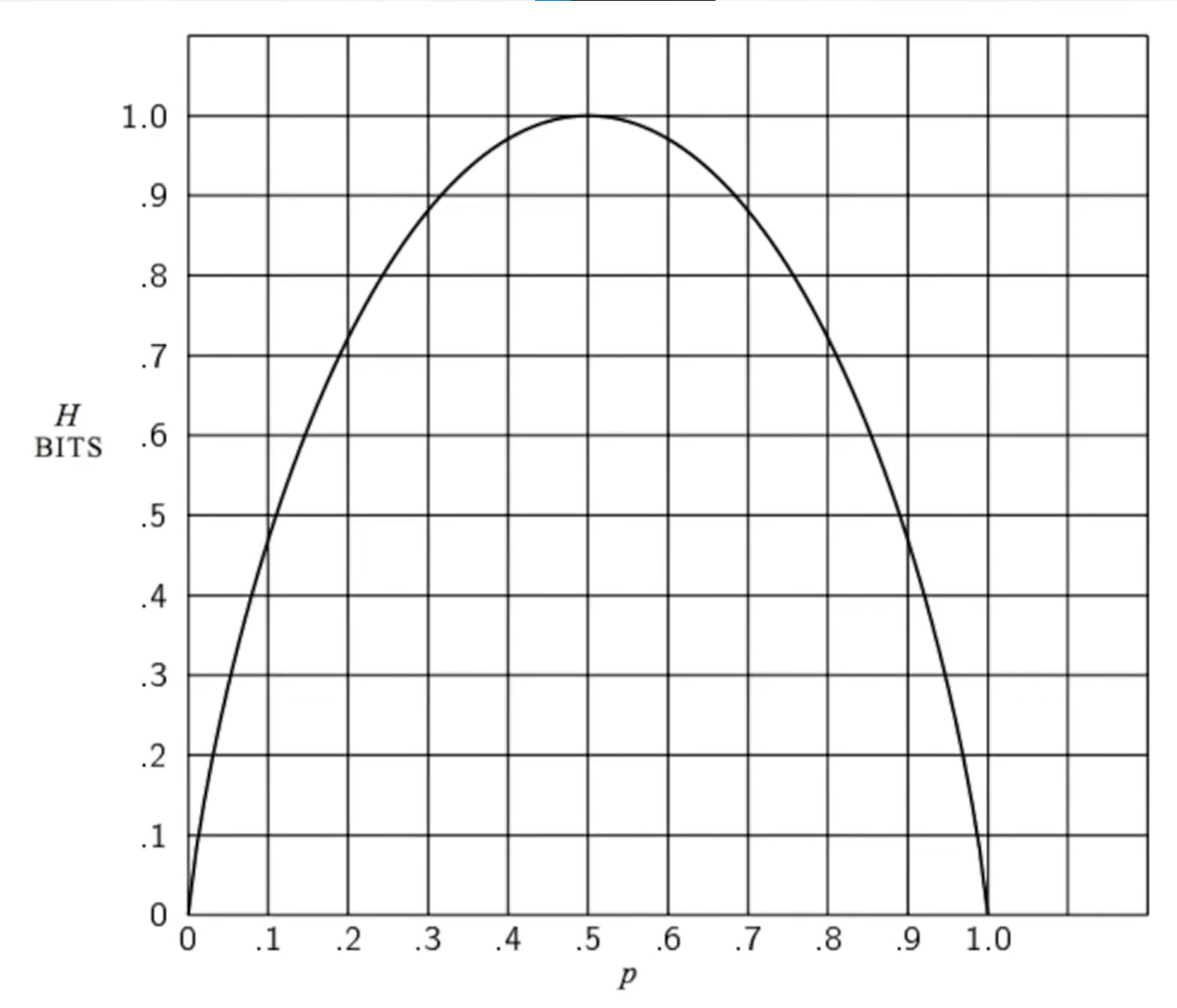
• Why is entropy relevant for decision trees? How is $H(p_1,p_2)$ defined?

  We use entropy to determine the importance of attributes.

  A lower entropy is better because it means we have to ask less questions (less testing = shallower tree) to reach a decison.

  Information gain measured with entropy

  Entropy measures uncertainty of the occurence of a random variable in [shannon] or [bit].

  Entropy of a random variable $A$ with values $v_k$ each with probability $P(v_k)$ is defined as:

  H(A)=∑kP(vk)log⁡2(1P(vk))=−∑kP(vk)log⁡2(P(vk))H(A) = \sum_k P(v_k)\log_2 \biggl( \frac{1}{P(v_k)} \biggl)= - \sum_k P(v_k)\log_2(P(v_k))H(A)=k∑​P(vk​)log2​(P(vk​)1​)=−k∑​P(vk​)log2​(P(vk​))

  Entropy is at its maximum when all outcomes are equally likely.

  

  Entropy of a boolean random variable

  Boolean random variable $V$ : Variable is true with probability $q$ and false with $(1-q)$ .

  Same formula as above.

  B(q)=−(q⋅log⁡2(q)+(1−q)⋅log⁡2(1−q))B(q)=-(q\cdot \log_2(q)+(1-q)\cdot \log_2(1-q))B(q)=−(q⋅log2​(q)+(1−q)⋅log2​(1−q))

Learning

• overfitting, ways to avoid it

  Overfitting

  occurs when a function is too closely aligned to training set - then it does not generalize well.

  To lower likelyhood of overfitting:

  • Ockham's Razor: "Maximize simplicity under consistency"

    We choose the most simple consistent hypothesis. - simpler hypotheses might generalize better

  • Choose hypothesis-space with lower expressiveness

  • remove unneccessary attributes from input

  • use more examples

  • Cross-Validation : Use part of the data for training, part for testing

• What is inductive learning?

  analytical / deductive learning : going from general rule to more specific and efficient rule

  Inductive Learning : discovering the general rule from examples

  • Ignores prior knowledge

  • Assumes a deterministic, observable "environment"

  • Assumes examples are given (selection of examples for training set is challenging)

  • In its simplest form: learning a function from examples

  • Assumes agent wants to learn

• What is a learning curve? In which 2 cases is it not optimal?

  Learning curve = % correct on test set when using $h$

  Learning curve depends on realizability of the target function.

  Non-realizability can be due to

  • missing attributes

  • too restrictive hypothesis space (e.g.,linear function)

  • redundant expressiveness (e.g., loads of irrelevant attributes)

  

• Learning agents

  Goal: making agents improve themselves by studying their own experiences

  Learning instead of programming because designers

  1. can't foresee all the situations the agent might be in

  2. can't foresee all the environment changes

  3. don't know the solution

  Utility Agent → Learning Agent

  Learning Agent = performance element + learning element

  Each component from the utility agent can be learned

  • actions $\mapsto$ their causing conditions

  • percept sequence $\mapsto$ relevant world properties

  • prior knowledge about world

  • Utility function: world states, actions $\mapsto$ their desirability

  • Goals that maximize the agents utility

  

  

  • Example: Taxi

    Performance element knowledge about driving

    Critic reactions of customer / other drivers / pedestrians / bikers / police

    Learning element create rules - ie. not to turn steering wheel to quickly, break softly etc.

    Problem generator try brakes on slippery road, push back with side (wing) mirror only

• Learning agent components

  

  Performance element

  Everything in between sensors (input) and actuators (output) abstracted away.

  Takes in percepts and chooses actions.

  Critic

  Feedback on performance (based on a fixed performance standard).

  Learning element LE

  Change "knowledge components" of agent (problem generator and performance element - independent of agents architecture).

  Problem generator

  suggest actions for new experiences to learn from - based on learning goals

  ---

  Designing a learning element

  Design is defined by:

  • performance element type

  • functional component model that describes what actions do (we learn this)

  • representation mathematical model for functional component

  • available feedback

  Examples:

  

Neural Networks

• construct a neural network: $\equiv, \wedge, \oplus, \downarrow, \uparrow, (A\wedge (\neg B))$

  Activation function:

  $g(x)=\left\{\begin{array}{ll}1 & \text { if } x \geq 1, \\0 & \text { otherwise }\end{array}\right.$

  ---

  

  

  • Alternative activation functions

    Activation function:

    $g(x)=\left\{\begin{array}{ll}1 & \text {if ~} \frac{1}{3} \cdot x \geq 2 \\0 & \text {otherwise }\end{array}\right.$

    

    

    

• neuron unit

  Mathematical Model of Neuron

  McCulloch and Pitts (1943)

  The inputs stay the same, only the weights are changed.

  

  Each unit has a dummy input $a_0 = 1$ with the weight $w_{0,j}$ .

  The unit $j$ 's output activation $a_j$ is

  aj=g(inj)=g(∑i=0nwi,jai)a_j = g(in_j) = g\biggl( \sum_{i=0}^n w_{i,j}a_i \biggl)aj​=g(inj​)=g(i=0∑n​wi,j​ai​)

  Where $g$ is an activation function :

  perceptron hard threshhold $g(x)=\left\{\begin{array}{ll}1 & \text { if } x \geq 0 \\0 & \text { otherwise }\end{array}\right.$

  sigmoid perceptron logistic function $g(x) = \frac{1}{1+e^{-x}}$

• activation functions

  Determine a threshhold, that makes the neuron fire if it is reached.

  We use:

  • step function / hard limiter

  • linear function / treshold function

  • sigmoid function

  

• Advantages and disadvantages of neural networks / learning by observation

  Advantages and Disadvantages of Neural Networks

  Pros

  • Less need for determining relevant input factors

  • Inherent parallelism

  • Easier to develop than statistical methods

  • Capability to learn and improve

  • Quite good for complex pattern recognition tasks

  • Usable for "unstructured" and "difficult" input (e.g., images)

  • Fault tolerance

  Cons

  • Choice of parameters (layers, units for network) requires skill

  • Requires sufficient training material

  • Resulting hypotheses cannot be understood easily

  • Knowledge implicit (subsymbolic representation)

  • Verification and behavior prediction is difficult (if not impossible)

  Challenges

  • Interpretability

  • Explainability

  • Trustworthiness

  • Robustness (adversarial examples)

  • Combining symbolic and subsymbolic approaches

• Perceptron learning rule

  We train the weights for each scalar output seperately.

  The network stays the same, we want to learn the right weights. We learn the weights for each output in isolation.

  ---

  We want to learn $f(\mathbf x)$

  $h_{\mathbf{w}}(\mathbf{x}) = g(in)$ for unit $u_i$

  $\text{Err}=\left(y-h_{\mathbf{w}}(\mathbf{x})\right)$

  $\operatorname{Loss}(\mathbf{w})={\left(y-h_{\mathbf{w}}(\mathbf{x})\right)}^{2}$

  $\Delta=\operatorname{Err}_{i} ~\cdot ~g^{\prime}(i n_{i})$

  We want the minimal loss, through gradient search on $\mathbf w$ :

  We want to find the partial derivative of the loss function for each weight $w_i$ :

  ∂∂wiLoss(w)=−2⋅(y−hw(x))undefined=Err⋅g′(ini)undefined=Δ⋅xi\frac{\partial }{\partial w_{i}}\text {Loss}(\mathbf w)=-2 \cdot \underbrace{\underbrace{(y-h_{\mathbf{w}}(\mathbf{x}))}_{=\text{Err}} \cdot g^{\prime}(i n_i)}_{=\Delta} \cdot x_{i}∂wi​∂​Loss(w)=−2⋅=Δ=Err(y−hw​(x))​​⋅g′(ini​)​​⋅xi​

  wi←wi+α⋅(y−hw(x))⋅g′(ini)⋅xiw_i\larr w_i + \alpha \cdot (y-h_{\mathbf{w}}(\mathbf{x})) \cdot g^{\prime}(i n_i) \cdot x_{i}wi​←wi​+α⋅(y−hw​(x))⋅g′(ini​)⋅xi​

  ---

  1. Perceptron learning rule (Hard threshold)

     The hard thershold can't be derived.

     For each example $(\mathbf{x}, y)$ :

     wi←wi+α(y−hw(x))⋅xiw_i \larr w_i + \alpha(y-h_{\mathbf{w}}(\mathbf{x})) \cdot x_iwi​←wi​+α(y−hw​(x))⋅xi​

     • How does exactly it work?

       We have our currect output $h_{\vec w}$ and the output of the examples $y \in \{0,1\}$ with a given $\vec x$ .

       • $y = h_{\vec w}(\vec x)$

         Our weights are correct. $w_i$ stays unchanged.

       • $y=1$ and $h_{\vec w}(\vec x) = 0$

         Our weights are incorrect. We want to make $h_{\vec w}(\vec x) = 1$

         If $x_i$ is positive $\rarr w_i$ gets increased

         If $x_i$ is negative $\rarr w_i$ gets decreased

       • $y=0$ and $h_{\vec w}(\vec x) = 1$

         Our weights are incorrect. We want to make $h_{\vec w}(\vec x) = 0$

         If $x_i$ is positive $\rarr w_i$ gets decreased

         If $x_i$ is negative $\rarr w_i$ gets increased

  2. Gradient decend rule (Soft threshold)

     For each example $(\mathbf{x}, y)$ : (Both are equivalent)

     wi←wi+α⋅(y−hw(x))⋅hw(x)(1−hw(x))undefined=Δ⋅xiw_{i} \leftarrow w_{i}+\alpha \cdot \underbrace{ \left(y-h_{\mathbf{w}}(\mathbf{x})\right) \cdot h_{\mathbf{w}}(\mathbf{x})\left(1-h_{\mathbf{w}}(\mathbf{x})\right) }_{=\Delta} \cdot x_{i}wi​←wi​+α⋅=Δ(y−hw​(x))⋅hw​(x)(1−hw​(x))​​⋅xi​

• What is backwards propagation? How does it work for inner nodes?

  💡

  The index $k$ ranges over nodes in the output layer. The index $j$ ranges over nodes in the hidden layer.

  We want to learn the function

  input$\mathbf x =(x_1, x_2, \dots, x_n)$

  output$\mathbf{h}_{\mathbf{w}}(\mathbf{x}) = (a_k,a_{k+1}, \dots a_n)$

  We have a training set with examples $(\mathbf x, \mathbf y)$ .

  $\mathbf x =(x_1, x_2, \dots, x_n)$

  $\mathbf{y} = (y_1, y_2, \dots, y_n)$

  We want to minimize the loss (= the sum of gradient losses for all output nodes).

  ∂∂wkLoss⁡(w)=∂∂wk∣y−hw(x)∣2=∂∂wk∑k(yk−ak)2=∑k∂∂wk(yk−ak)2\frac{\partial}{\partial w_k} \operatorname{Loss}(\mathbf{w})= \textcolor{grey}{ \frac{\partial}{\partial w_k}\left|\mathbf{y}-\mathbf{h}_{\mathbf{w}}(\mathbf{x})\right|^{2}=\frac{\partial}{\partial w_k} \sum_{k}\left(y_{k}-a_{k}\right)^{2} } =\sum_{k} \frac{\partial}{\partial w_k}\left(y_{k}-a_{k}\right)^{2}∂wk​∂​Loss(w)=∂wk​∂​∣y−hw​(x)∣2=∂wk​∂​k∑​(yk​−ak​)2=k∑​∂wk​∂​(yk​−ak​)2

  Problem: dependency

  We can not learn the weights the same way we did for the single layer network.

  The multilayer network has a hidden layer and the output functions are nested functions that contain the nodes behind them.

  The error for the hidden layers is not clear - we want to be able to push errors back.

  output nodes

  Each term in the final summation is computed as if the other outputs did not exist.

  Same rule as in the single-layer perceptron.

  $\text{Err}_k =$ the $k$ th component of the vector $(\mathbf{y}-\mathbf{h}_{\mathbf{w}}(\mathbf x))$

  $\Delta_k = \text{Err}_k \cdot g^{\prime}(in_j)$

  wj,k←wj,k+α⋅Δk⋅ajw_{j,k} \leftarrow w_{j,k}+\alpha \cdot \Delta_k \cdot a_{j}wj,k​←wj,k​+α⋅Δk​⋅aj​

  wj,k←wj,k+α⋅Errk⋅g′(inj)undefined=Δk⋅ajw_{j,k} \leftarrow w_{j,k}+\alpha \cdot \underbrace{ \text{Err}_k \cdot g^{\prime}(in_j)}_{=\Delta_k} \cdot a_{j}wj,k​←wj,k​+α⋅=Δk​Errk​⋅g′(inj​)​​⋅aj​

  wj,k←wj,k+α⋅(y−hw(x))k⋅g′(∑iwi,kai)undefined=Δk⋅ajw_{j,k} \leftarrow w_{j,k}+\alpha \cdot \underbrace{ (\mathbf{y}-\mathbf{h}_{\mathbf{w}}(\mathbf x))_k \cdot g' \bigl( \sum_{i} w_{i,k}a_i \bigl)}_{=\Delta_k} \cdot a_{j}wj,k​←wj,k​+α⋅=Δk​(y−hw​(x))k​⋅g′(i∑​wi,k​ai​)​​⋅aj​

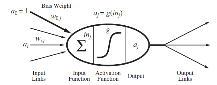
  Where$w_{j,k}$stands for the weight between the nodes$j$and$k$.

  The idea is that the hidden node$j$is "responsible" for some fraction of the error$\Delta_k$in each of the output nodes to which it connects.

  Thus, the$\Delta_k$values are divided according to thestrength of the connection between the hidden node and the output node and are propagated back to provide the $\Delta_j$values for the hidden layer.

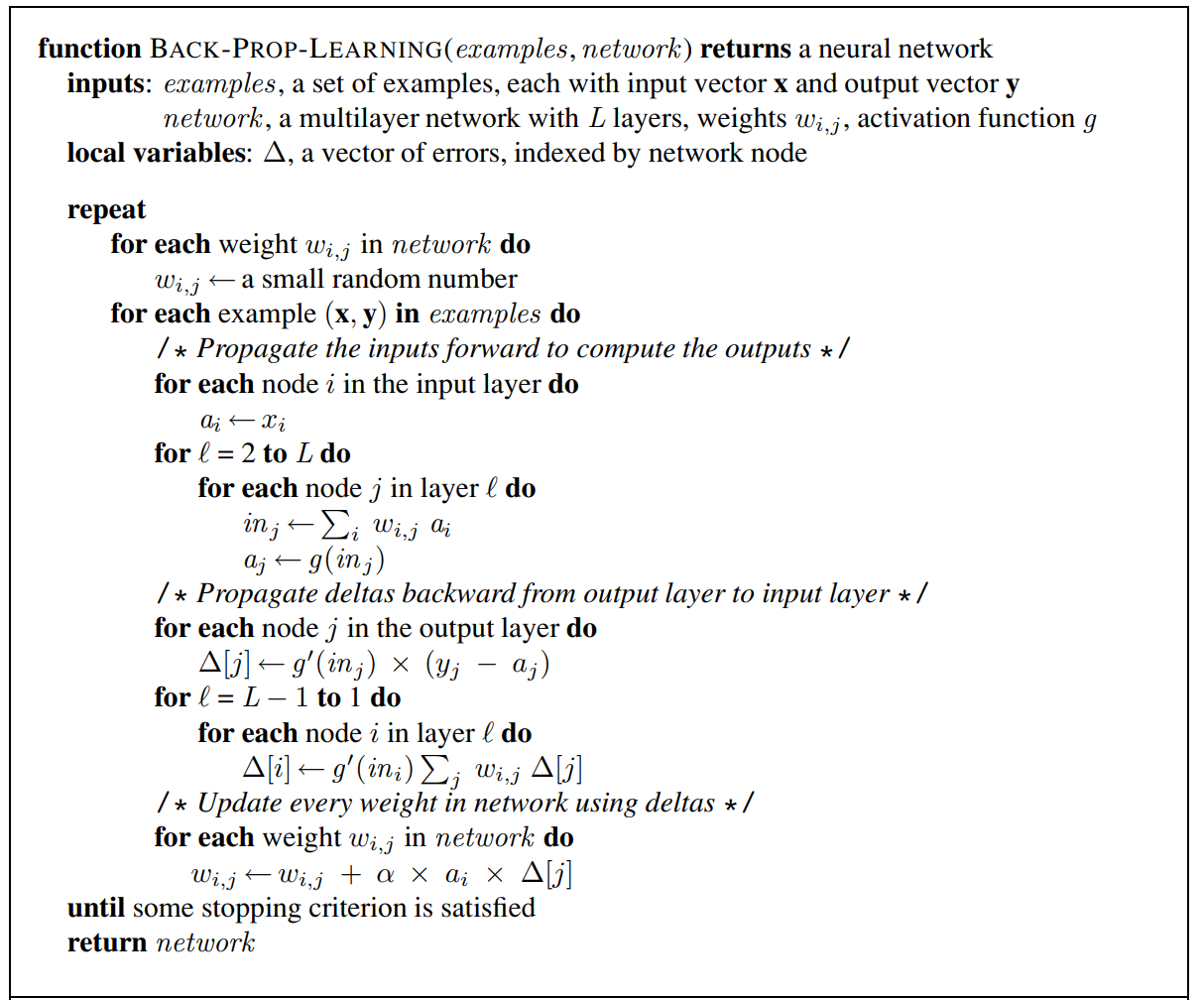
  hidden nodes: Back-propagation

  We back propagate the errors from the output to the hidden layers.

  Δj=g′(inj)∑kwj,k⋅Δk\Delta_{j}=g'(i n_{j}) \sum_{k} w_{j, k} \cdot\Delta_{k}Δj​=g′(inj​)k∑​wj,k​⋅Δk​

  Δj=g′(∑i=0nwi,jai)undefined=g′(inj)⋅∑kwj,k⋅(y−hw(x))k⋅g′(∑iwi,kai)undefined=Δk\Delta_{j}=\underbrace{ g' \bigl( \sum_{i=0}^n w_{i,j}a_i \bigl) }_{=g'(in_j)} \cdot\sum_{k} w_{j, k} \cdot \underbrace{ (\mathbf{y}-\mathbf{h}_{\mathbf{w}}(\mathbf x))_k \cdot g' \bigl( \sum_{i} w_{i,k}a_i \bigl)}_{=\Delta_k}Δj​==g′(inj​)g′(i=0∑n​wi,j​ai​)​​⋅k∑​wj,k​⋅=Δk​(y−hw​(x))k​⋅g′(i∑​wi,k​ai​)​​

  wi,j←wi,j+α⋅Δj⋅aiw_{i,j} \larr w_{i,j} + \alpha \cdot \Delta_j\cdot a_iwi,j​←wi,j​+α⋅Δj​⋅ai​

  The back propagation algorithm:

  

  • The math behind back propagation

    ∂∂wLoss⁡(w)=∂∂w∣y−hw(x)∣2=∂∂w∑k(yk−ak)2=∑k∂∂w(yk−ak)2=∑k∂∂wLossk\frac{\partial}{\partial w} \operatorname{Loss}(\mathbf{w})=\frac{\partial}{\partial w}\left|\mathbf{y}-\mathbf{h}_{\mathbf{w}}(\mathbf{x})\right|^{2}=\frac{\partial}{\partial w} \sum_{k}\left(y_{k}-a_{k}\right)^{2}=\sum_{k} \frac{\partial}{\partial w}\left(y_{k}-a_{k}\right)^{2} =\sum_{k} \frac{\partial}{\partial w} \text{Loss}_k∂w∂​Loss(w)=∂w∂​∣y−hw​(x)∣2=∂w∂​k∑​(yk​−ak​)2=k∑​∂w∂​(yk​−ak​)2=k∑​∂w∂​Lossk​

    For the$k$th output nodes

    ∂Loss⁡k∂wj,k=−2(yk−ak)∂ak∂wj,k=−2(yk−ak)∂g(ink)∂wj,k=−2(yk−ak)g′(ink)∂ink∂wj,k=−2(yk−ak)g′(ink)∂∂wj,k(∑jwj,kaj)=−2(yk−ak)g′(ink)aj=−ajΔk\begin{aligned}\frac{\partial \textcolor{pink}{\operatorname{Loss}_{k}}}{\partial \textcolor{pink}{w_{j, k}}} &=-2\left(y_{k}-a_{k}\right) \frac{\partial a_{k}}{\partial w_{j, k}}=-2\left(y_{k}-a_{k}\right) \frac{\partial g\left(i n_{k}\right)}{\partial w_{j, k}} \\&=-2\left(y_{k}-a_{k}\right) g^{\prime}\left(i n_{k}\right) \frac{\partial i n_{k}}{\partial w_{j, k}}\\&=-2\left(y_{k}-a_{k}\right) g^{\prime}\left(i n_{k}\right) \frac{\partial}{\partial w_{j, k}}\left(\sum_{j} w_{j, k} a_{j}\right) \\&=-2\left(y_{k}-a_{k}\right) g^{\prime}(i n_{k}) a_{j}\\&=-a_{j} \Delta_{k}\end{aligned}∂wj,k​∂Lossk​​​=−2(yk​−ak​)∂wj,k​∂ak​​=−2(yk​−ak​)∂wj,k​∂g(ink​)​=−2(yk​−ak​)g′(ink​)∂wj,k​∂ink​​=−2(yk​−ak​)g′(ink​)∂wj,k​∂​(j∑​wj,k​aj​)=−2(yk​−ak​)g′(ink​)aj​=−aj​Δk​​

    With $\Delta_k$ defined as before.

    For the$j$th hidden nodes

    ∂Loss⁡k∂wi,j=−2(yk−ak)∂ak∂wi,j=−2(yk−ak)∂g(ink)∂wi,j=−2(yk−ak)g′(ink)∂ink∂wi,j=−2Δk∂∂wi,j(∑jwj,kaj)=−2Δkwj,k∂aj∂wi,j=−2Δkwj,k∂g(inj)∂wi,j=−2Δkwj,kg′(inj)∂inj∂wi,j=−2⋅Δk⋅wj,k⋅g′(inj)⋅∂∂wi,j(∑iwi,jai)=−2Δk⋅wj,k⋅g′(inj)ai=−ai⋅Δj\begin{aligned}\frac{\partial \operatorname{Loss}_{k}}{\partial w_{i, j}} &=-2\left(y_{k}-a_{k}\right) \frac{\partial a_{k}}{\partial w_{i, j}}=-2\left(y_{k}-a_{k}\right) \frac{\partial g\left(i n_{k}\right)}{\partial w_{i, j}} \\&=-2\left(y_{k}-a_{k}\right) g^{\prime}\left(i n_{k}\right) \frac{\partial i n_{k}}{\partial w_{i, j}}=-2 \Delta_{k} \frac{\partial}{\partial w_{i, j}}\left(\sum_{j} w_{j, k} a_{j}\right) \\&=-2 \Delta_{k} w_{j, k} \frac{\partial a_{j}}{\partial w_{i, j}}=-2 \Delta_{k} w_{j, k} \frac{\partial g\left(i n_{j}\right)}{\partial w_{i, j}} \\&=-2 \Delta_{k} w_{j, k} g^{\prime}(i n_{j}) \frac{\partial i n_{j}}{\partial w_{i, j}} \\&=-2 \cdot\Delta_{k}\cdot w_{j, k} \cdot g^{\prime}(i n_{j})\cdot \frac{\partial}{\partial w_{i, j}}(\sum_{i} w_{i, j} a_{i}) \\&=-2 \Delta_{k}\cdot w_{j, k}\cdot g^{\prime}(i n_{j}) a_{i}\\&=-a_{i}\cdot \Delta_{j}\end{aligned}∂wi,j​∂Lossk​​​=−2(yk​−ak​)∂wi,j​∂ak​​=−2(yk​−ak​)∂wi,j​∂g(ink​)​=−2(yk​−ak​)g′(ink​)∂wi,j​∂ink​​=−2Δk​∂wi,j​∂​(j∑​wj,k​aj​)=−2Δk​wj,k​∂wi,j​∂aj​​=−2Δk​wj,k​∂wi,j​∂g(inj​)​=−2Δk​wj,k​g′(inj​)∂wi,j​∂inj​​=−2⋅Δk​⋅wj,k​⋅g′(inj​)⋅∂wi,j​∂​(i∑​wi,j​ai​)=−2Δk​⋅wj,k​⋅g′(inj​)ai​=−ai​⋅Δj​​

    With $\Delta_j$ defined as before.

• What is deep learning, when does it work well, where are its shortcomings?

  Deep Learning

  Deep learning: Hierarchical structure learning - Artificial neural network with many layers.

  Feature extraction and learning (un)supervised

  Problem: requires lots of data

• Which functions can be represented with single and multi-layer perceptrons?

  One hidden layer all continuous function, can be as precise as one wants

  Two hidden layers all functions

  Single-layer feed-forward neural networks (Perceptrons)

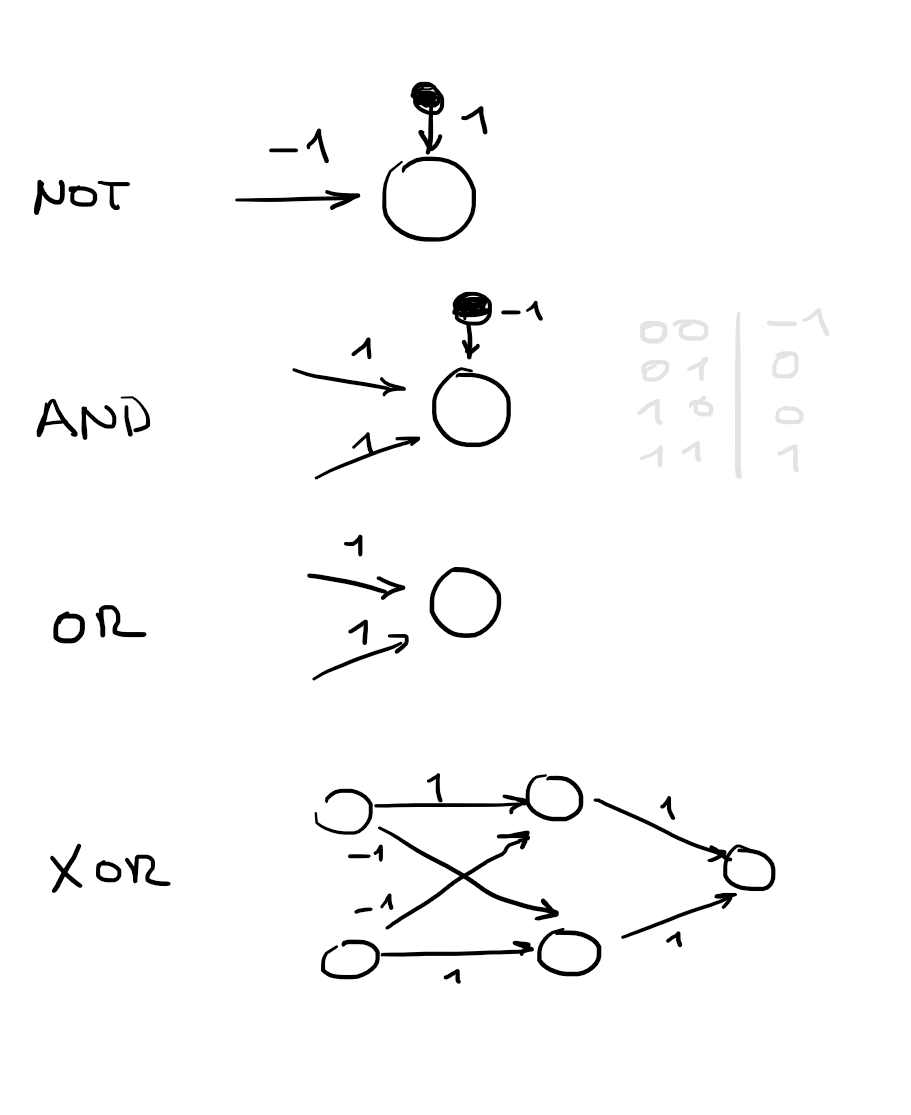
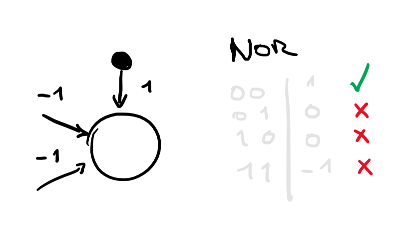
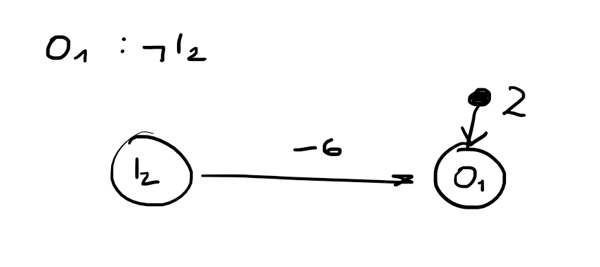
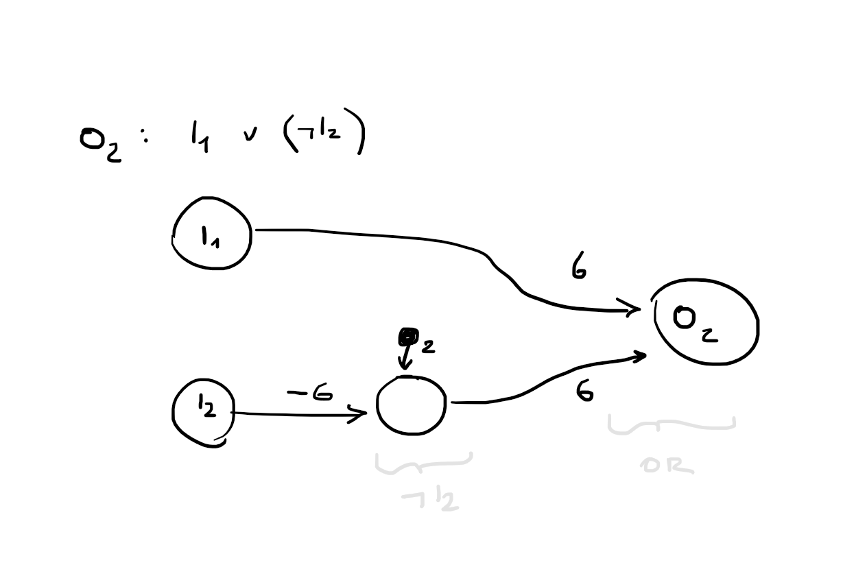
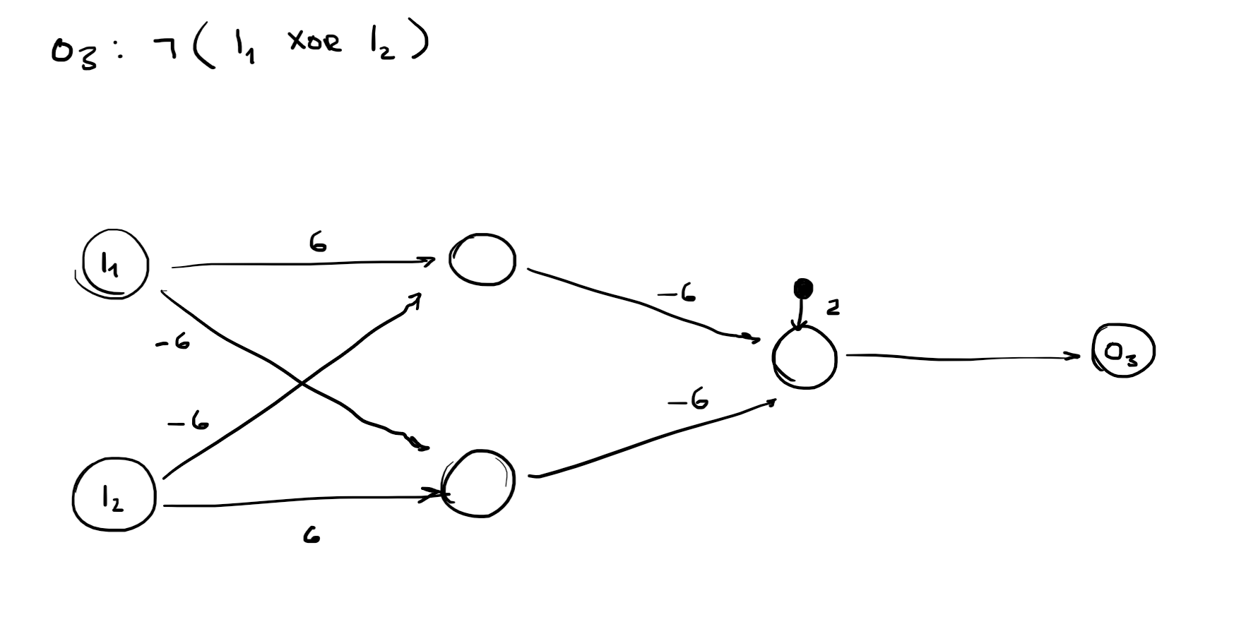
  No hidden layers: Always represents a linear separator in the input space - therefore can not represent the XOR function.

  Multilayer feed-forward neural networks

  With a single, sufficiently large hidden layer (2 layers in total), it is possible to represent any continuous function of the inputs with arbitrary accuracy.

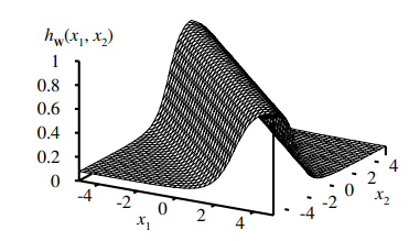
  • in depth

    Above we see a nested non-linear function as the solution to the output.

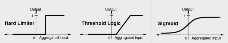
    With the sigmoid function as $g$ and a hidden layer, each output unit computes a soft-thresholded linear combination of several sigmoid functions.

    For example, by adding two opposite-facing soft threshold functions and thresholding the result, we can obtain a "ridge" function.

    

    Combining two such ridges at right angles to each other (i.e., combining the outputs from four hidden units), we obtain a "bump".

    

    With more hidden units, we can produce more bumps of different sizes in more places.

  With two hidden layers, even discontinuous functions can be represented.

CSP

• Cryptographic puzzle as a CSP

    E G G
  + O I L
  -------
  M A Y O

  Defined as a constraint satisfaction problem:

  $X = \{E, G, O,I,L,A,Y, X_1, X_2, X_3\}$

  $D=\{0,1,2,3,4,5,6,7,8,9\}$

  Constraints:

  Each letter stands for a different digit: $\operatorname{Alldiff}(E,G,O,I,L,A,Y)$

  $\begin{array}{l} G+L=O+10 \cdot X_{1} \\ X_{1}+G+I=Y+10 \cdot X_{2}, \\ X_{2}+E+O=A+10 \cdot X_{3}, \\ X_{3}=M \end{array}$

  The $X_1, X_2, X_3$ variables stand for the digit that gets carried over into the next column by the addition. Therefore $X_1$ stands for $10$ in our unknown numeric system, $X_2$ stands for $100$ , $X_3$ stands for $1000$ .

• Explain Backtracking Search for CSPs - why isn't it efficient?

  CSPs as standard search problems

  If we do not consider commutativity we have $n!d^n$ leafs else we have $d^n$ leafs.

  The order of the assignments has no effect on the outcome. - Choosing a single variable variable in each tree level.

  Backtracking search algorithm

  Uninformed search algorithm (not effective for large trees).

  Depth-first search:

  1. chooses values for one unassigned variable at a time - does not matter which one because of commutativity.

  2. tries all values in the domain of that variable

  3. backtracks when a variable has no legal values left to assign.

  Because its ineffective we use heuristics / General-purpose methods for backtracking search.

• backtracking heuristics for choosing variables and values

  Variable ordering: fail first

  • Minimum remaining values MRV

  • degree heuristic - (used as a tie breaker)

  Value ordering: fail last

  • least-constraining-value - a value that rules out the fewest choices for the neighbouring variables in the constraint graph.

• Does a CSP with $n$ variables and $d$ values in its domain have $O(d^n)$ possible assignemnts?

  Yes - this is because we are considering the commutativity of operatins and pick a single variable to assign for each tree level.

Classical Planning

• STRIPS vs. ADL

  STRIPS

  • only positive literals in states

  • closed-world-assumption: unmentioned literals are false

  • Effect $P \wedge \neg Q$ means add $P$ and delete $Q$

  • only ground atoms in goals

  • Effects are conjunctions

  • No support for equality or types

  ADL

  • positive and negative literals in states

  • open-world-assumption: unmentioned literals are unknown

  • Effect $P \wedge \neg Q$ means add $P$ and $\neg Q$ delete $Q$ and $\neg P$

  • goals contain $\exists$ quantor

  • goals allow conjunction and disjunction

  • conditional effects are allowed: $P:E$ means $E$ is only an effect if $P$ is satisfied

  • equality and types built in

• formalize a STRIPS action

  $\text{Action}(\text{Drive}(car, from, to),$

  $\text{PRECOND:}~\text{At}(car, from)\wedge \text{Car}(car) \wedge \text{Location}(from) \wedge \text{Location}(to)$

  $\text{EFFECT:} ~\text{At}(car, to) \wedge \neg\text{At}(car, from)~~)$

• Planning: What 3 problems occur in reasoning about actions?

  Reasoning about the results of actions

  frame problem ... what are things that stay unchanged after action?

  would require a lot of axioms to describe.

  ramification problem ... what are the implicit effects?

  ie.: passengers of a car move with it

  qualification problem ... what are preconditions for actions?

  deals with a correct conceptualisation of things (no answer).

  ie.: finding the right formalization of a human conversation

Classical Planning with state space search

• explain POP algorithm

  Partial-order Planning

  Order is not specified: can place to actions into a plan without specifying which one comes first.

  Search in space of partial-order-plans.

  Components of a plan

  1. actions set

     not actions in the world but actions on plans . ie. adding an ordering to the plan, ...

  2. ordering constraints set

     $A \prec B$ Must be free of contradictions/cycles$(A \prec B) \wedge (B\prec A)$

  3. casual links set

     $A \stackrel{p}{\longrightarrow} B$ Executing action $A$ achieves precondition $p$ for action $B$ .

     Means $p$ must remain $\text{true}$ from time of action $A$ to the time of action $B$ .

     else there is a conflict$C$ .

     ie:$\text {RightSock} \stackrel{\text {RightSockOn}}{\longrightarrow} \text {RightShoe}$

  4. open preconditions set

     Minimizing open preconditions (= preconditions not achieved by an action in the plan)

  Algorithm

  Defines execution order of plan by searching in the space of partial-order plans.

  Returns a consistent plan : without cycles in the ordering constraints and conflicts in the casual links.

  1. Initiating empty plan

     only contains the actions:

     $\text{Start}$ no preconditions, effect has all literals, all preconditions are open

     $\text{Finish}$ no open preconditions, effect has no literals.

     ordering constraint: $\text { Start} \prec \text {Finish}$

     no casual links

  2. Searching

     2.1 successor function: repeatedly choosing next possible state.

     Chooses an open precondition $p$ of action $B$ and generates a successor plan (subtree) for every consistent way of choosing an action $A$ that achieves $p$ .

     2.2 enforce consistency by defining new casual links in the plan:

     $A \stackrel{p}{\longrightarrow} B, \space A \prec B$

     If$A$is new:$\text{Start} \prec A \prec\text{Finish}$

     2.3 resolve conflicts

     add $(B\prec C) \wedge (C\prec A)$

     2.4 goal test

     because only consistent plans are generated - just check if preconditions are open.

     If goal not reached, add successor states

  Example

• Does POP it only produce consistent plans?

  Yes - because only consistent plans are generated the goal test is checking if any preconditions are open. If the goal is not reached it adds successor states.

• all types of state space search algorithms

  Totally ordered plan searches

  in strictly linear order.

  The state space is finite without function symbols - any graph search algorithm can be used.

  Variants:

  • progression planing: initial state $\rarr$ goal

  • regression planing: initial state $\larr$ goal

    (possible because of declarative representation of PDDL and strips)

  Partial-order Planning

  Order is not specified: can place to actions into a plan without specifying which one comes first.

  Search in space of partial-order-plans.

• consistent plans (in partial order planning) and solutions

  solutionto a declared planning-problem= a plan

  • Any action sequence that when executed in the initial state - results in a state that satisfies the goal.

  • Every action sequence that maintains the partial order is a solution.

    (The in POP algorithm the goal is therefore only defined by not having open preconditions)

  Consistent actions

  Chosen actions should not undo the progress made.

  Consistent plans (in partial order planning)

  Must be free of contradictions / cycles in the ordering constraint set : $(A \prec B) \wedge (B\prec A)$

  Must be free of conflicts in the casual links set : precondition $p$ must remain $\text{true}$ if $A \stackrel{p}{\longrightarrow} B$ .

• order constraint and when does it lead to problems?

  $A \prec B$ Action $A$ must be executed before action $B$ .

  Must be free of contradictions/cycles : $(A \prec B) \wedge (B\prec A)$

Utility

• risk aversion: What would the risk averse agent prefer $\text{U}(L)$ or $\text{U}(S_{\text{EMV}(L)})$ ?

  as we gain more money, its utility does not rise proportionally.

  The Utility for getting your first million dollars is very high, but the utility for the additional million is smaller.

  For the risk averse agent:

  $U(L) < U(\textcolor{pink}{S_{EMV(L)}})$

  the utility of being faced with that lottery $<$ than the utility of being handed the expected monetary value of the lottery with absolute certainty

• expected utility, maximum estimated utility

  Expected Utility (average)

  Its impicit that $s'$ can follow from the current state $s$ .

  $E U(a \mid \mathbf{e})=\sum_{s^{\prime}} P(\operatorname{RESULT}(a)=s^{\prime} \mid a, \mathbf{e}) \cdot U(s^{\prime})$

  Sum of: Probability of state occuring after action times its utility

  Principle of maximum expected utility MEU

  rational agent should choose the action that maximizes the agents expected utility

  $\text { action }=\underset{a}{\operatorname{argmax}} \space E U(a \mid \mathbf{e})$

• The axioms of utility theory

  Constraints on rational preferences of an agent

  Notation:

  $A \succ B$ agent prefers state $A$ over state $B$

  $A \sim B$ agent is indifferent between state $A$ and state $B$

  $A \succsim B$ one of the above

  Constraints

  1. Orderability

     The agent must have a preference.

     $(A \succ B) \space \textsf{xor} \space (B \succ A) \space \textsf{xor} \space (A \succsim B)$

  2. Transivity

     $(A \succ B) \wedge(B \succ C) \Rightarrow(A \succ C)$

  3. Continuity

     $A \succ B \succ C \Rightarrow \exists p:\space[p, A ; 1-p, C] \sim B$

  4. Substitutability

     If agent is indifferent to $A$ and $B$ then agent is indifferent to complex lotteries with same probabilities.

     $A \sim B \Rightarrow[p, A ; 1-p, C] \sim[p, B ; 1-p, C]$

  5. Monotonicity

     Agent prefers a higher probability of the state that it prefers.

     $A \succ B \Rightarrow(p>q \Leftrightarrow[p, A ; 1-p, B] \succ[q, A ; 1-q, B])$

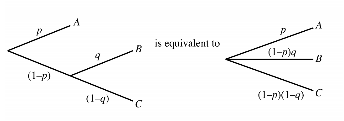
  6. Decomposability

     Compound lotteries can be reduced to simpler ones.

     $[p, A ; 1-p,[q, B ; 1-q, C]] \sim[p, A ;(1-p) q, B ;(1-p)(1-q), C]$

  

  If an agent violates these axioms it will exhibit irrational behaviour.

  • Example: intransitive preferences

    $A \succ B \succ C \succ A$

    Agent can be induced to give away all its money:

    Agent has $A$

    1. We offer $A$ + 1 cent for $C$ (agent accepts)

    2. We offer $B$ + 1 cent for $C$ (agent accepts)

    3. We offer $A$ + 1 cent for $B$ (agent accepts)

    We repeat all over again.

    

Making decisions

• Components of a decision network

  = influence diagrams.

  General framework for rational decisions. Return the action with highest utility.

  Decision networks are an extension of Bayesian networks.

  Presents:

  1. current state

  2. possible actions

  3. resulting state from actions

  4. utility of each state

  Node types:

  Chance nodes (ovals) Random variables, uncertainty - Bayes Network

  Decision nodes (rectangles) Decision maker has choice of action

  Utility nodes (diamonds) Utility function

  

VPI

• value of information - Can it be calculated without additional information?

  Value of Information

  $\text{value = }(\text{ avg. best action before obtaining}) - (\text{avg. best action after obtaining})$

  • Example: Oil Company

    There are $n$ different indistinguishable blocks.

    $\frac{1}{n}$ blocks has oil worth $C$ dollars.

    Others are worthless.

    Blocks cost $\frac{C}{n}$ dollars.

    How much is the information whether a block 3 has oil or not worth to the company?

    • $P(\text{block has oil}) = \frac{1}{n}$

      If the block has oil, the company will buy it $-\frac{C}{n}$ and then profit $C$ dollars:

      $C − \frac{C}{n} = \frac{(n-1) \cdot C}{n}$

    • $P(\text{block has no oil}) = \frac{1}{n}$

      If the block has no oil, the company will buy a different block because the probability of finding oil in other ones changes from $\frac{1}{n}$ to $\frac{1}{n-1}$ .

      Average profit: of $\frac{C}{n-1} - \frac{C}{n} = \frac{C}{n(n-1)}$ dollars.

    We then calculate the expected / average profit with the information:

    $\frac{1}{n} \cdot \frac{(n-1) \cdot C}{n} + \frac{1}{n-1} \cdot \frac{C}{n(n-1)}= \frac{C}{n}$

    Which is equal to the price we would be for a block if we would not have had this information.

  • Example: Oil Company (simplified)

    There are $n$ boxes.

    Opening a box costs costs $\frac{C}{n}$ dollars.

    $\frac{1}{n}$ boxes contains $C$ dollars, others are worthless.

    How much is the information whether box 3 has oil or not worth to the company?

    • $P(\text{box has prize}) = \frac{1}{n}$

      Then we will pay the price to open it and take the money inside: $C − \frac{C}{n}$

    • $P(\text{box has no prize}) = \frac{1}{n}$

      Then we will open another box - the probability of finding the prize changes from $\frac{1}{n}$ to $\frac{1}{n-1}$ and on average we make $\frac{C}{n-1} - \frac{C}{n}$ dollars.

    We then calculate the average profit with the information:

    $P(\text{box has prize}) \cdot (C − \frac{C}{n} ) + P(\text{box has prize}) \cdot (\frac{C}{n-1} - \frac{C}{n}) = \frac{C}{n}$

    Therefore this information has a value of $\frac{C}{n}$ .

    This is what it would cost us to find it out ourselves and we are willing to pay someone $<\frac{C}{n}$ to figure it out for us.

  Value of perfect information VPI(= expected value of information)

  Lets say the exact evidence $e_j$ (= perfect information) of the random variable $E_j$ is currently unknown.

  We define:

  Best action$\alpha$before learning$e_j = E_j$under all actions$\textcolor{pink}a$

  $E U(\alpha \mid \mathbf{e})=\max _{\textcolor{pink}a} \sum_{s^{\prime}} P(\operatorname{RESULT}(\textcolor{pink}a)=s^{\prime} \mid \textcolor{pink}a, \mathbf{e}) \cdot U(s^{\prime})$

  Best action$\alpha_{e_j}$after learning$e_j = E_j$under all actions$\textcolor{pink}a$

  $E U(\alpha_{e_{j}} \mid \mathbf{e}, e_{j})=\max _{\textcolor{pink}a} \sum_{s^{\prime}} P(\operatorname{RESULT}(\textcolor{pink}a)=s^{\prime} \mid \textcolor{pink}a, \mathbf{e}, e_{j}) \cdot U(s^{\prime})$

  Value of learning the exact evidence is the cost of discovering it for ourselves under $\mathbf{e}$ by averaging over all possible values $e_{jk}$ of $E_j$ .

  VPIe(Ej)=(∑kP(Ej=ejk∣e)⋅EU(αejk∣e,Ej=ejk))−EU(α∣e)V P I_{\mathbf{e}}(E_{j})=\left(\sum_{k} P(E_{j}=e_{j k} \mid \mathbf{e}) \cdot EU(\alpha_{e_{j k}} \mid \mathbf{e}, E_{j}=e_{j k})\right)-E U(\alpha \mid \mathbf{e})VPIe​(Ej​)=(k∑​P(Ej​=ejk​∣e)⋅EU(αejk​​∣e,Ej​=ejk​))−EU(α∣e)

  VPI is non-negative

  In the worst case, one can just ignore the received information.

  $\forall \mathbf{e}, E_{j} \quad V P I_{\mathbf{e}}\left(E_{j}\right) \geq 0$

  Important: this is about the expected value, not the actual value.

  Additional information can lead to plans that turn out to be worse than the original plan.

  Example: a medical test that gives a false positive result may lead to unnecessary surgery; but that does not mean that the test shouldn’t be done.

  VPI is non-additive

  The VPI can get higher or lower as new information gets aquired as combined information can have different effects.

  $\operatorname{VPI}_{\mathbf{e}}\left(E_{j}, E_{k}\right) \neq V P I_{\mathbf{e}}\left(E_{j}\right)+\operatorname{VPI}_{\mathbf{e}}\left(E_{k}\right)$

  VPI is order independent

  $V P I_{\mathbf{e}}\left(E_{j}, E_{k}\right)=V P I_{\mathbf{e}}\left(E_{j}\right)+V P I_{\mathbf{e}, e_{j}}\left(E_{k}\right)=V P I_{\mathbf{e}}\left(E_{k}\right)+V P I_{\mathbf{e}, e_{k}}\left(E_{j}\right)$