Utility
Utility Theory
Utility theory and probability theory (for decision-theoretic agents)
deals with uncertainty, conflicting goals, maximizing utility.
Decision theory
deals with desireability of immediate outcomes in an episodic environment.
Non-deterministic, in partially observable environments
Outcome defined by random variable .
Probability of outcome with given observations .
Utility function
desireability of state
Expected Utility (average utility value)
Its impicit that can follow from the current state .
Sum of: Probability of state occuring after action times its utility
Principle of maximum expected utility MEU
rational agent should choose the action that maximizes the agents expected utility
Axioms of Utility theory
Constraints on rational preferences of an agent - MEU can be derived from these constraints.
Notation:
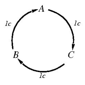
agent prefers state over state
agent is indifferent between state and state
one of the above
Lottery
Set of possible outcomes for each action.
Lottery
outcome (can be atomic or another lottery = complex lottery )
probability
Constraints
- Orderability
The agent must have a preference.
- Transivity
- Continuity
If there is a probability for which the agent would be indifferent to
getting with absolute certainty
or with probability and with
- Substitutability
If agent is indifferent to and then agent is indifferent to complex lotteries with same probabilities.
- Monotonicity
Agent prefers a higher probability of the state that it prefers.
- Decomposability
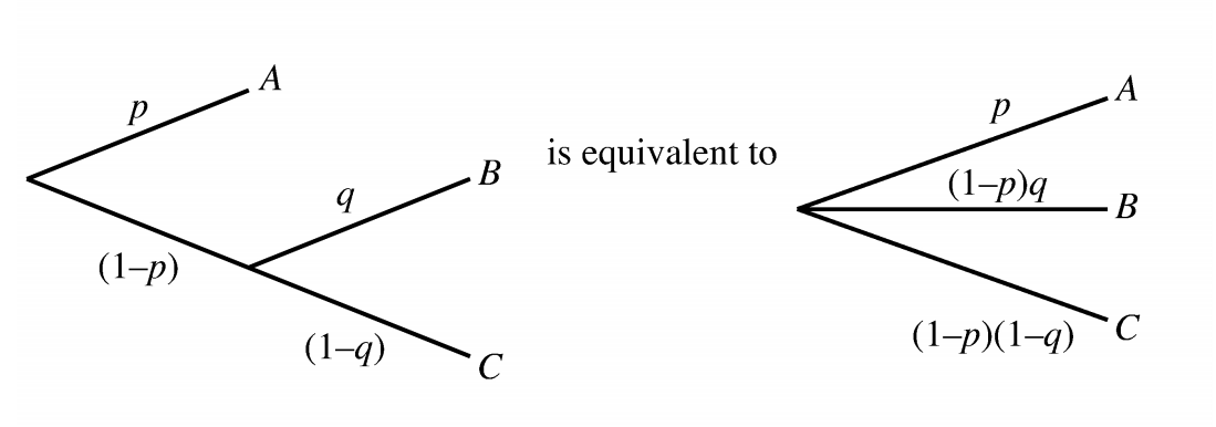
Compound lotteries can be reduced to simpler ones.

If an agent violates these axioms it will exhibit irrational behaviour.
Preference constraints → Utility Function
Existence of utility function
If agent is rational, there exists a real-valued function so that
The agents behavior would not change if:
(affine transformation) with constants
It is therefore not something unique .
The numbers do not matter - this is a value / ordinal utility function .
Expected utility of a lottery
is the sum of the probability of each outcome times its utility.
Utility assessment and Utility scales
We want to build a decision theoretic system that helps the agent make decisions.
Examples for utility scales
micromort - one-in-a-million chance of death
value that people place on their own lifes.
ie. 1 micromort is equivalent to 20 USD (1980s money).
QALY - quality-adjusted life year
one QALY equates to one year in perfect health.
is an indicator for the time-trade-off (TTO): to choose between being ill vs. being healthy but having a shorter life expectancy.
ie. on average, kidney patients are indifferent between living two years on a dialysis machine and one year at full health
Preference elicitation
Testing / observing agent and finding out its underlying utility function.
There are no absolute values for utility function - we try to create it:
best possible prize
worst possible catastrophe
Normalized utilities
best possible prize
worst possible catastrophe
Utility of Money
Utility measure = agents total net assets.
Agents have monotonic preference for more money - they prefer having more.
That says nothing about preferences between lotteries involving money.
Expected monetary value EMV
The EMV (money made on average) ≠ the utility of it, because of:
- the agents current net asset
- risk-averseness of agent
Certainty equivalent
reminder
the utility of being faced with that lottery than the utility of being handed the expected monetary value of the lottery with absolute certainty
Most people will accept about $400 in alternative to playing a gamble that gives $1000 half the time and $0 the other half.
In this case:
- certainty equivalent of the lottery $400
- expected monetary value EMV $500
Insurance premium
= EMV - certainty equivalent of a lottery
is based on risk aversion.
Risk neutral
For small changes in wealth relative to the current wealth, almost any curve will be approximately linear.
An agent that has a linear curve is said to be risk-neutral. This justifies the axioms of probability.
